Outflows initiated by magnetically modified spherical accretion onto black hole

Bestin James 1 , Vladimír Karas 2 , Agnieszka  Janiuk 1

  • 1 Center for Theoretical Physics Polish Academy of Sciences, Warsaw
  • 2 Astronomical Institute of the Czech Academy of Sciences, Prague

Abstract

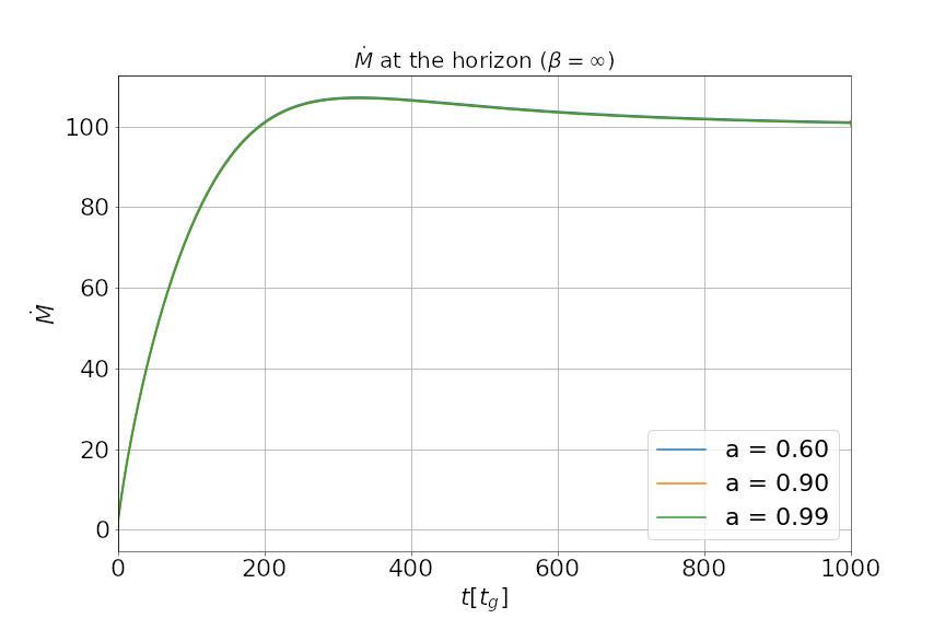
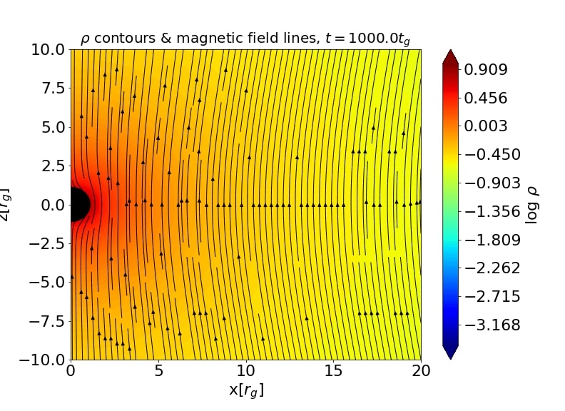
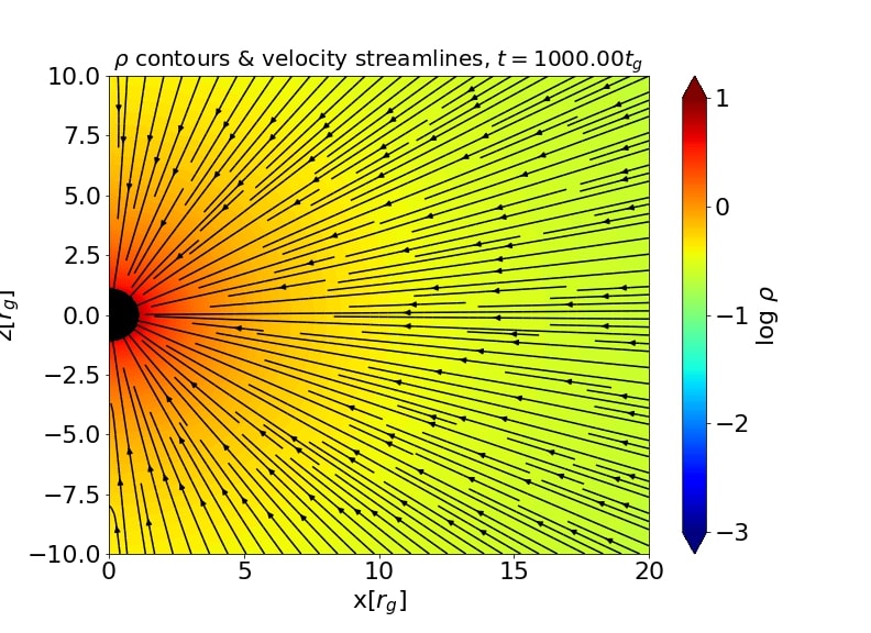
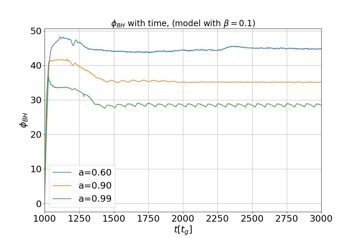
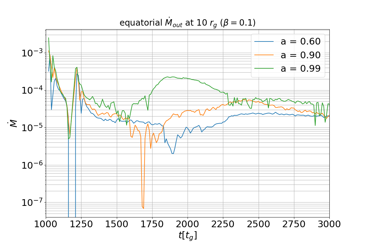
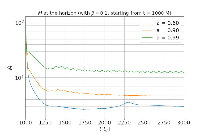
Cosmic plasma is largely ionized and magnetized due to the presence of electric currents in the highly conductive environment near black holes. The plasma in the vicinity of a black hole is attracted to it by the immense gravity and often results in an accretion flow that is accompanied by ejection. As the accretion proceeds, the frozen-in plasma brings along with it more magnetic flux to the black hole horizon which can eventually result in a high magnetic pressure relative to the gas pressure near the black hole horizon. We model outflows driven by a large-scale magnetic field in the vicinity of a rapidly rotating black hole by general relativistic relativistic magnetohydrodynamic simulations. We initialize our simulations with an initially spherical accretion profile and a uniform magnetic field in the Kerr geometry. The magnetic field lines frozen into the plasma are rapidly accreted onto the black hole as the simulations begin canceling the initial Meissner-like expulsion due to the rapid rotation of the black hole. We notice magnetic reconnection events near the equatorial plane which drives an outflow in our models. We also notice repetitive fluctuations of the accretion rate and the emergence of velocity vortices in the accretion flow which can affect the rate of outflows.

Introduction

Various observational studies point towards the idea that an accreting black hole acts as the central engine of astrophysical objects such as active galactic nuclei (AGN) and gamma-ray bursts. The accretion of plasma onto the central compact object due to its gravitational force produces various observable effects including the relativistic jets and outflows in the form of winds. It is appropriate to assume that plasma at large-scales is magnetized due to its environment. In this work we focus on the equatorial outflows in an accreting plasma around a central black hole mediated by the presence of large-scale magnetic fields. Such outflows are recently considered to explain the observed properties of M87*, with an in-fall of matter at a larger radius and an ejection disc at a smaller radius [1]. In this work we are interested in gradually evolving the structure of the magnetic field and mass flow in the regions near to the black hole horizon in the presence of a large-scale uniform magnetic field (Wald, 1974) [2]. We use an initially spherically symmetric inflow, given by the Bondi (1952) solution [3], as the initial stationary solution and evolve it with time. 

Conclusions

  • In this work, we focused on the transition between two extreme states of accretion, where a Wald-type uniform initial seed field aligned with the black hole rotation axis comes in contact with a radial Bondi-type mass inflow. The plasma drags the field lines to the black hole horizon, and at the same time become influenced and partly expelled by the evolution of the magnetic field. Our model serves as a test solution that demonstrates the rapid disappearance of magnetic expulsion as the conducting plasma starts to get accreted. As this happens, the magnetic field lines are bent in the radial direction and start to reconnect along the equatorial plane thus accelerating an outflow in a direction perpendicular to the rotation axis of the black hole. We can suggest that such backflows are a generic feature that can occur in different accreting systems.
  • For future work, we plan to investigate the effects of an asymptotically uniform magnetic field inclined with respect to the rotation axis of the black hole and evolve the non-axisymmetric 3D configuration. This is interesting as this will involve tangled magnetic field structures and the effect of this on the outflow rates and the inward accretion rate are to be investigated. We can thus investigate different angles between the black hole spin and the magnetic field direction and look further into their effect on the equatorial dynamics of accretion flows now governed by the magnetic reconnection-driven turbulence.


Numerical setup

Code Setup

We model accretion onto a black hole in a fixed Kerr metric. The metric is not evolved in time with the assumption that the accreted mass is negligible in comparison to the black hole mass over the timescale considered. We assume the ideal MHD and evolve its equations with the numerical code \(\texttt{HARM}\). We use a modified version of the \(\texttt{HARM}\) code which is a conservative and shock capturing scheme for evolving the equations of ideal magnetohydrodynamics in general relativity (GRMHD) [4,5,6]. So the magnetic field lines are frozen into the plasma. The code follows the evolution of the accretion flow by solving the continuity, energy-momentum conservation and induction equations in the GRMHD scheme

$$ \nabla_\mu(\rho u^{\mu})= 0 $$

$$ \nabla_\mu(T^{\mu\nu}) = 0 $$

$$ \nabla_\mu(u^\nu b^\mu - u^\mu b^\nu) = 0 $$

where \(u^{\mu}\) is the four-velocity of the gas, \(u\) is the internal energy, \(\rho\) is the gas density, \(p\) is the gas pressure, and \(b^{\mu}\) is the magnetic four-vector. \(T\) is the stress-energy tensor which comprises matter and electromagnetic parts, \(T^{\mu \nu} = T^{\mu \nu}_{\mathrm{gas}} + T^{\mu \nu}_{\mathrm{EM}}\). The magnetic field \(B\) is connected to the magnetic four-vector in such a way that \(b^i = (B^i + b^tu^i)/u^t\) where \(b^t = B^iu^{\mu}g_{i\mu}\).

The outer boundary of the computational domain is set at \(10^5~r_g\) and the inner boundary is located at \(0.98~r_{H}\), i.e. a fraction inside the event horizon radius, for the corresponding value of black hole spin \(a\). The 2D grid domain has a resolution of \(600 \times 512\) in the (\(r,\theta\)) directions. For the 3D grid, we use a resolution of \(288 \times 256 \times 128\) in the \((r, \theta, \phi)\) directions. We use a uniform angular resolution for the grid in our models. The adiabatic index is assumed to be that of an ideal gas with \(\gamma = 4/3\). We use the plasma \(\beta\) parameter which is defined as the gas to magnetic pressure ratio (\(p_\mathrm{gas} /p_\mathrm{mag}\)) to initially set the maximum magnetic field strength in the models as the field is enabled, where, \(p_\mathrm{gas} = (\gamma - 1)u_\mathrm{max}\) and \(p_\mathrm{mag} = b_\mathrm{max}^2/2\). 

Models - initial setup

We begin all our models with a uniform density over the entire computational grid and with no magnetic field around. This configuration is evolved with time, as we see the gas starts accreting to the black hole, and the mass accretion rate rises and reaches a quasi-steady value. The evolution of the accretion rate at this stage is plotted in Figure 1. At this point (at \(1000~t_g\) in our models), we introduce the magnetic field.


Figure 1: Mass accretion rate rate on the black hole horizon for the initial part of the simulation before the magnetic field is turned on (\(\beta = \infty\)). The value initially grows and saturates to a quasi-stationary value as the time proceeds. It is in geometric units which can be scaled with the black hole mass \(M\). The accretion rate at this stage for all the black hole spin values are the same as we use the same initial conditions for the density.

The magnetic field in our models is prescribed according to the solution for an asymptotically uniform field parallel to the rotatation axis around a Kerr black hole, given by the Wald (1974) solution [2]. This field can be prescribed by the only non-vanishing components of the vector potential,

$$  A_t = B_0 a [r\Sigma^{-1}(1+\cos^2\theta)-1]  $$

$$ A_{\phi} = B_0[\frac{1}{2}(r^2+a^2)-a^2r\Sigma^{-1}(1+\cos^2\theta)]\sin^2\theta, $$

with \(\Sigma = r^2 + a^2\cos^2\theta\).

At the point in time when the magnetic field is turned on, the plasma distribution posses a Bondi-type steady accretion rate it acquired from the earlier part of the simulation. At the instance we turn on the magnetic field, the field lines are expelled from the black hole horizon similar to the standard Meissner effect. This is shown in Figure 2(a). This effect is expected for any rotating black hole with the maximally spinning case showing the highest degree of expulsion [7, 8]. The velocity streamlines at the instance when we introduce the magnetic field is depicted in Figure 2(b), showing the purely radial inflow at the this time.

Figure 2(a): Initial state of magnetic field lines overplotted on top of density contours in the domain, at the instance when the magnetic field is turned on (at t = 1000 M; for the model b01.a90.2D - as given in Table 1) (Time evolution in next section).

Figure 2(b): Initial state of velocity streamlines overplotted on top of the density contours in the domain, at the instance when the magnetic field is turned on (at t = 1000 M; for the model b01.a90.2D - as given in Table 1) (Time evolution in next section).

References

[1] R. Blandford, N. Globus, MNRAS 514, 5141 (2022).

[2] R. M. Wald, Phys. Rev. D 10, 1680 (1974).

[3] H. Bondi, MNRAS 112, 195 (1952).

[4] C. F. Gammie, J. C. McKinney, G. T ́oth, ApJ 589, 444 (2003).

[5] S. C. Noble, C. F. Gammie, J. C. McKinney, L. Del Zanna, ApJ 641, 626 (2006).

[6] A. Janiuk, K. Sapountzis, J. Mortier, I. Janiuk, Supercomputing Frontiers and Innovations 5, 86–102 (2018).

[7] J. Bicak, V. Janis, MNRAS 212, 899 (1985).

[8] A. R. King, J. P. Lasota, W. Kundt, Phys. Rev. D 12, 3037 (1975).

[9] A. Janiuk, B. James, A&A 668, A66 (2022).

Discussion of results

\begin{array}{lcccccc} % columns, alignment for each \hline \text{Model} & \beta_{max} & a & \langle\dot M_{\rm in,H}\rangle_t & \langle\phi_{\rm BH}\rangle_t & \langle\dot M_{{\rm out,10r_{\it g}}}\rangle_t & \langle\dot M_{{\rm out,10r_{\it g}}}\rangle_t \\ & & & \text{(code units)} & & \text{(code units)} & (M_{\odot} \text{yr}^{-1}) \\ \hline \text{b1.a0.2D} & 1.0 & 0 & 4.58 & 43.08 & 3.00 \times 10^{-5}& 1.060 \times 10^{-7} \\ \text{b1.a60.2D} & 1.0 & 0.60 & 2.18 & 41.95 & 3.07 \times 10^{-5}& 1.084 \times 10^{-7} \\ \text{b1.a90.2D} & 1.0 & 0.90 & 2.30 & 35.06 & 4.82 \times 10^{-5}& 1.703 \times 10^{-7} \\ \text{b1.a90.2D} & 1.0 & 0.90 & 2.30 & 35.06 & 4.82 \times 10^{-5}& 1.703 \times 10^{-7} \\ \text{b1.a99.2D} & 1.0 & 0.99 & 4.41 & 28.72 & 8.11 \times 10^{-5}& 2.864 \times 10^{-7} \\ \text{b05.a0.2D} & 0.5 & 0 & 3.06 & 45.73 & 2.36 \times 10^{-5}& 8.325 \times 10^{-8} \\ \text{b05.a60.2D} & 0.5 & 0.60 & 1.92 & 43.44 & 2.45 \times 10^{-5}& 8.666 \times 10^{-8} \\ \text{b05.a90.2D} & 0.5 & 0.90 & 2.44 & 35.57 & 3.99 \times 10^{-5}& 1.410 \times 10^{-7} \\ \text{b05.a99.2D} & 0.5 & 0.99 & 4.56 & 28.88 & 6.87 \times 10^{-5}& 2.429 \times 10^{-7} \\ \text{b01.a0.2D} & 0.1 & 0 & 3.60 & 46.78 & 2.16 \times 10^{-5} & 7.645 \times 10^{-8}\\ \text{b01.a60.2D} & 0.1 & 0.60 & 3.60 & 44.67 & 2.81 \times 10^{-5} & 9.941 \times 10^{-8} \\ \text{b01.a90.2D} & 0.1 & 0.90 & 5.53 & 35.68 & 4.29 \times 10^{-5} & 1.515 \times 10^{-7} \\ \text{b01.a99.2D} & 0.1 & 0.99 & 14.34 & 29.04 & 9.18 \times 10^{-5}& 3.243 \times 10^{-7} \\ %\vspace{2\baselineskip}\\ %------ 3D models ----% \text{b01.a90.3D} & 0.1 & 0.90 & 3.94 & 43.36 & 8.50 \times 10^{-5} & 3.003 \times 10^{-7}\\ \text{b01.a99.3D} & 0.1 & 0.99 & 9.34 & 32.41 & 12.65 \times 10^{-5} & 4.468 \times 10^{-7}\\ \hline \end{array} \\

Table 1: Summary of models investigated. The models are parameterized by the initial maximum plasma \(\beta\) and the dimensionless Kerr parameter \(a\). The time-averaged mass accretion rate at the horizon and the equatorial mass outflow rate at 10 \(r_g\) are computed after the magnetic field is turned on (i.e. from 1000 \(t_g\)). The outflow rate given in the last column is the estimated value in physical units considering our model of mass ejection for the M87 central engine.

The models studied in this work are summarized in Table 1 and their names in the first column reflect the parameter values used for them and the setup (2D or 3D). The time evolution of the density and the magnetic field lines as well as the velocity field are already presented in the previous section.

Figure 3: The evolution of magnetic flux on the black hole horizon with time for the 2D models with \(\beta = 0.1\) and with different spin values from time \(t = 1000~t_g\)

Figure 4: The equatorial mass outflow rate with time at 10 \(r_g\), after the magnetic field is turned on, for the 2D models with \(\beta = 0.1\) and different spin values.

Figure 5: The evolution of inward mass accretion rate at the black hole horizon with time, after the magnetic field is turned on, for the 2D models with \(\beta = 0.1\) and different spin values.

Figure 3 shows the time-evolution of magnetic flux on the black hole horizon for the models with initial maximum \(\beta = 0.1\). The magnetic flux on the black hole horizon is quantified by

$$ \phi_{BH}(t) = \frac{1}{2\sqrt{\dot{M}}} {\int_{\theta} \int_{\phi} \mid{B^{r}(r_{H},t)}\mid dA_{\theta \phi}} $$

The initial flux is very high as the initial uniform field strength is 10 times higher than the gas pressure. As the accretion proceeds, this flux still keeps high with values of \(\phi_{BH} \sim 30 - 45\). Values in this range can suggest that the accretion is magnetically arrested and further inflow of matter can occur through magnetic reconnections and interchange instabilities.

  • The mass outflows are sustained in time as can be seen from the outflow rates plot shown in Figure 4, computed at \(10~r_g\). This is the case with all our models, with the highly magnetized models showing the highest outflow rates when averaged over time as given in Table 1.
  • Figure 5 shows the inward mass accretion rate at the black hole horizon for the models with \(\beta = 0.1\). We can notice some quasi-periodic fluctuations in the mass accretion rate as well as the magnetic flux on the horizon (in Figure 4) and these effects seem to depend on the black hole spin.
  • In the last column of Table 1, we give the estimated mass outflow rate for the realistic system of M87 considering its known physical parameters. Since we use a unit convention of \(G = c = M = 1\) in the code, the length and time units for the simulations results are given by \(L_\mathrm{unit} = GM/c^2\) and \(T_\mathrm{unit} = GM/c^3\) respectively. So the length and time values can be converted to physical units by using the relevant value of the black hole mass and the accretion rate can be calculated by considering a density scaling for the accreting medium under consideration. More details of this computation can be found in one of our previous article [9].
  • Analytic models similar to the configuration we are considering, in which a spherically symmetric inflow at a large radius and an ejection disk at a smaller radius, are recently considered to account for the observed variability in M87 [1].


Time evolution of models

Video 1: Time evolution of the density overplotted with magnetic field lines for the 3D model with initial \(\beta = 0.1\) and \(a=0.90\) on the equatorial (XY) slice.

Video 2: Time evolution of the density overplotted with magnetic field lines for the 3D model with initial \(\beta = 0.1\) and \(a=0.90\) on a poloidal (XZ) slice (with \(\phi =0\))

Video 3: Time evolution of the density overplotted with velocity streamlines for the 3D model with initial \(\beta = 0.1\) and \(a=0.90\) on the equatorial (XY) slice

Video 4: Time evolution of the density overplotted with velocity streamlines for the 3D model with initial \(\beta = 0.1\) and \(a=0.90\) on the poloidal (XZ) slice (with \(\phi =0\))

Links to the videos on YouTube: Video 1, Video 2, Video 3, Video 4.

The Videos 1-4 show the time evolution of the magnetic field lines and veloctiy streamlines on top of the density contors, for the model b01.a90.3D, as given in Table 1. They show the regions closer to the black hole up to \(30 r_g\) in equatorial and polar slices.


In the beginning of Video 2, we can notice the rapid dissappearance of the "Meissner-like" expulsion of magnetic filed lines as the accretion of matter proceeds. In the same video, it is also possible to notice the reconnection of mangetic field lines while being accreted into the black hole, in regions below \(5 r_g\). In Video 4, we can notice the velocity and density structures developed in the domain signifying the outflows in the equatorial region. In the same video, we also note the development of turbulence and velocity vortices in the flow.