Magritte, a 3D NTLE line radiative transfer code for imaging the circumstellar environment

Thomas Ceulemans 1

  • 1 Ku Leuven

Abstract

A central question in astrophysics pertains the origin of the chemical enrichment of the universe.
It is generally hypothesized that a major part of the chemical species originate from the circumstellar environment of stars. As the stars eject matter, it cools down in the circumstellar environment, allowing interesting chemistry to happen.
A wealth of different types of circumstellar environments have been observed, ranging from protoplanetary disks to wild AGB outflows. In all these regions, complex interactions between chemistry, hydrodynamics and radiation transfer take place. In order to properly understand the interactions, we need to model them. To compare these modeling efforts with actual images of astrophysical objects, accurate radiative transfer computations are required. To aid in these radiative transfer modeling efforts, we are continuing to develop Magritte, an open-source 3D line radiative transfer library. To ensure the performance of Magritte, the library has been written in c++. For ease of use, we support a simple python API. In this talk, we show how to apply Magritte to general models in order to generate synthetic spectra. To show the flexibility of Magritte, we compute synthetic spectra of two types of hydrodynamics models: particle-based and grid-based.

To summarize: The circumstellar environment is an important source of the chemical enrichment of the universe. In this talk, we use the line radiative transfer code Magritte to generate synthetic spectra from hydrodynamics models of the circumstellar environment, allowing us to compare these models to actual observations.

Magritte

Magritte is an open-source 3D NLTE line radiative transfer library. The basics of radiative transfer is given by the radiative transfer equation; the intensity in a specific direction changes because of material emitting or absorbing energy.

\hat{\boldsymbol{n}}\cdot \nabla I(x,\nu)=\eta(x,\nu)-\chi(x,\nu) I(x,\nu)
\text{In which } \hat{\boldsymbol{n}} \text{ is the direction, } I \text{ is the monochromatic specific intensity, } \eta \text{ is the total emissivity and } \chi \text{ is the total opacity.}

In line radiative transfer, a sharp frequency dependence is introduced, as light will be admitted/absorbed at specific frequencies, corresponding to energy transitions.

\eta_{ij}(x,\nu)=\frac{h\nu}{4\pi}n_i(x)A_{ij}\phi_{ij}(x, \nu)
\chi_{ij}(x,\nu)=\frac{h\nu}{4\pi}\left(n_j(x)B_{ji}-n_i(x)B_{ij}\right)\phi_{ij}(x, \nu)
\text{In which } \chi_{ij} \text{ is the line opacity, } \eta_{ij} \text{ is the line emissivity, } n_i \text{ are the populations of energy level i, } A_{ij}, B_{ij}, B_{ji} \text{ are the Einstein coefficients and } \phi_{ij} \text{ is the line profile function.}

In NLTE (non local thermodynamical equilibrium) radiative transfer, the radiation field influences the level populations ni as prescribed by the static equilibrium equations.

\sum_{ji} \left(n_jA_{ji}-(n_iB_{ij}-n_jB_{ji})J_{ij}\right)\nonumber\\ +\sum_{j=1}^N \left(n_iC_{ij}-n_jC_{ji}\right)=0
\text{In which the mean line intensity } J_{ij} \text{ is given by } J_{ij}(\boldsymbol{x})=\oint_{\Omega}\int_0^{+\infty} I(\hat{\boldsymbol{n}},\boldsymbol{x},\nu)\phi_{ij}(\nu)\text{d}\Omega \text{d}\nu \text{.}

An iterative process is thus required for NLTE line radiative transfer computations, as the intensity field influences the level populations ni which influences the opacities/emissivities used for computing the intensity.

Features

  • Python api
  • Online documentation
  • Written in C++ for performance
  • Automated testing procedure


Novel computational improvements

  • Computing optical depths in high velocity gradients
  • Adaptive Ng acceleration

Github repository

Documentation

Optical depths in large velocity gradients

Most discretizations of the radiative transfer equation use optical depths 𝜏, which are computed by numerically integrating the opacity over a distance increment Δx. The optical depth increment Δ𝜏(𝜈) on a small segment given by a single line at a specific frequency 𝜈 is then given by

\Delta \tau(\nu) = \int_0^{\Delta x} \chi_{ij}(x,\nu) dx
\text{In which } \chi \text{ is the opacity, which depends on the line profile function } \phi \text{.}

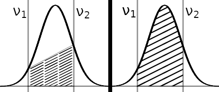
For small velocity gradients, it is sufficient to use the trapezoidal rule to discretize the integral. However, for larger velocity gradients, this discretization might be too coarse and can result in missing the peak of the line profile function, as illustrated in the figure below.

To avoid this issue, one can either split the discretization into more parts or one can exploit knowledge about the shape of the line profile function.

If we assume the shape of the line profile to be gaussian (similar derivations can be done for other shapes), we can split the opacity into a slowly varying part without the line profile χ̅ and the line profile function ϕ. We put the slowly varying part outside the integral and analytically integrate the line profile function to obtain

\Delta\tau(\nu)=\Delta x\left(\frac{\overline{\chi}_{ij}(x_0)+\overline{\chi}_{ij}(x_1)}{2}\right)\left(\frac{\text{Erf}(f(x_1))-\text{Erf}(f(x_0))}{2\Delta\nu}\right)
\text{In which } \Delta x = x_1 - x_0 \text{ is the position increment, } f(x)= \frac{\nu-\nu_l(x)}{\delta \nu} \text{ is the dimensionless line frequency, for which } \nu_l \text{ is the line frequency, } \delta\nu \text{ is the line width and } \Delta \nu \text{ is the frequency difference.}

Use cases of Magritte

Creating Magritte models: SPH

Creating Magritte models: Adaptive Mesh Refinement

Synthetic observations

Future work

3D line radiative transfer is computationally expensive. Thus we will implement GPU computing, making use of machine learning libraries.

  • Widespread support for accelerators (GPU's, ...)
  • Allows for sensitivity analysis using the computed gradients

Adaptive Ng acceleration

To compute line radiative transfer self-consistently, an iterative procedure is required. This procedure can be accelerated by using the linear extrapolation procedure known as Ng-acceleration (Ng 1974). The general idea is use data (e.g. level populations) from the N previous iterations to extrapolate the results.

However, the optimal value for this hyperparameter N is model dependent. To help with this choice, we introduce adaptive Ng acceleration. Instead of using a fixed amount of iterations N, we can allow the acceleration step to happen earlier based on whether the accelerated data converges faster than the non-accelerated results. As the extrapolated data no longer changes significantly, it is no longer useful to add an extra regular step before extrapolating.

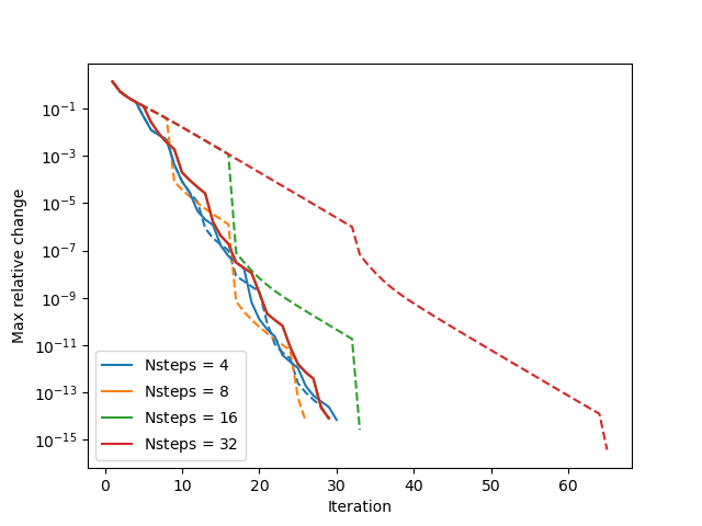
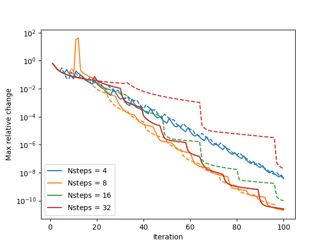
To illustrate the effect of adaptive Ng-acceleration, we used the Van Zadelhoff benchmarks (1D spherically symmetric collapsing cloud ; van Zadelhoff et al. 2002) to compare the adaptive Ng acceleration scheme with default Ng acceleration. We have plotted the convergence behavior in the figures below. For a given value of the hyperparameter N, adaptive Ng-acceleration results in similar or better convergence behavior compared to default Ng-acceleration.


Convergence results for the optically thin Van Zadelhoff 1a model. The dashed lines correspond to regular Ng acceleration, while the dotted lines correspond to adaptive Ng acceleration with the specified maximal number of steps in between extrapolation.

Convergence results for the optically thick Van Zadelhoff 1b model. The dashed lines correspond to regular Ng acceleration, while the dotted lines correspond to adaptive Ng acceleration with the specified maximal number of steps in between extrapolation.

Personal webpage

Synthetic observations with Magritte

Synthetic observation of an AMRVAC hydrodynamics model by Jan Bolte.