- The majority of massive stars belong to binary systems:
- Considerably affects the evolution of the stars;
- Offers possibilities to constrain the properties of the stars.
- Interesting systems: double-line spectroscopic eclipsing binaries
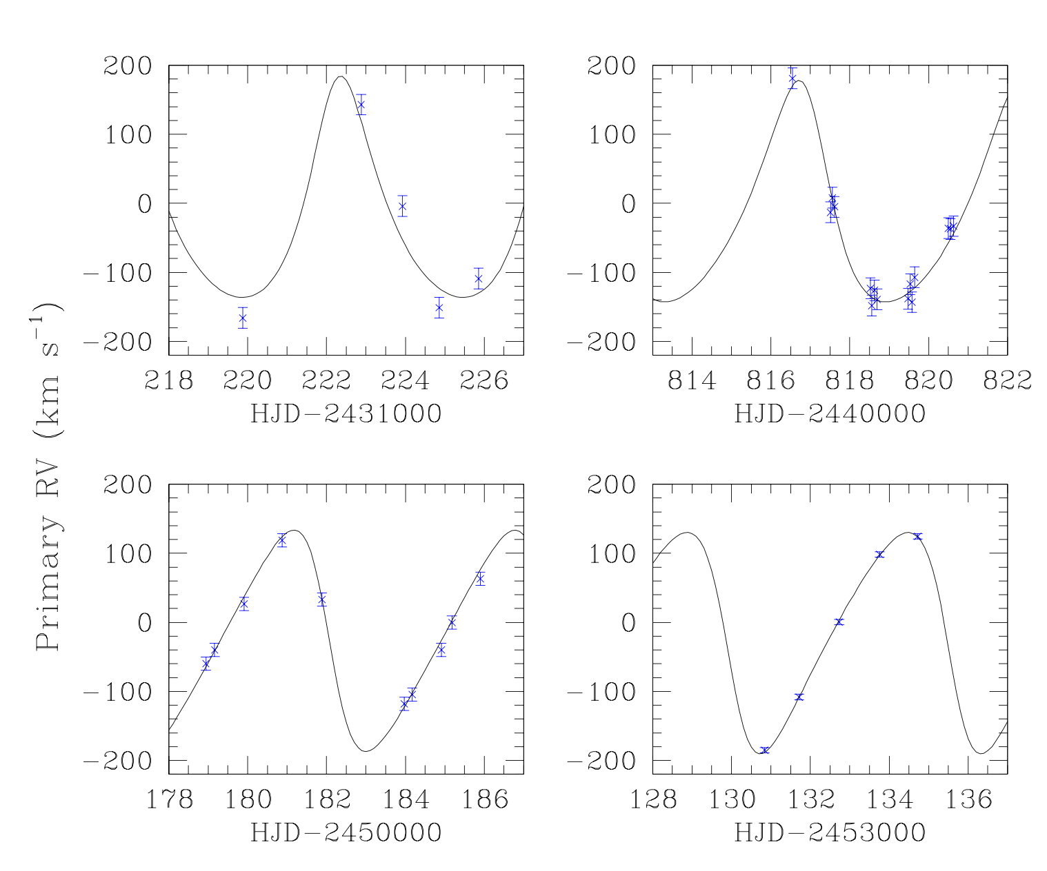
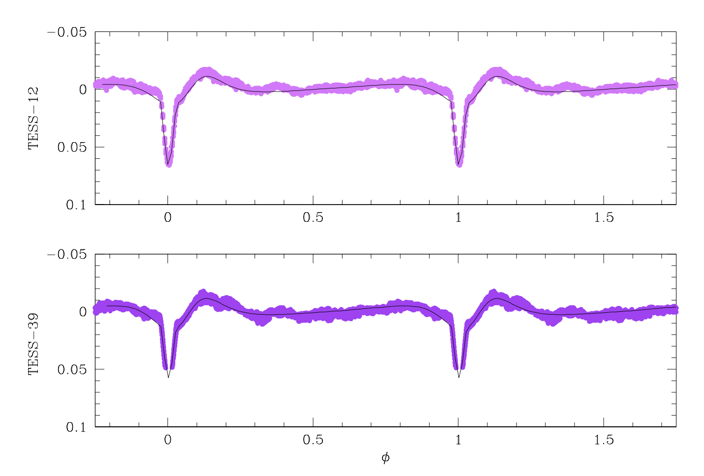
- Combine the photometric eclipses and the radial velocities obtained with spectroscopy;
- Determine the masses and radii of the stars in a model independent way.
- Most interesting systems: binaries showing a significant apsidal motion
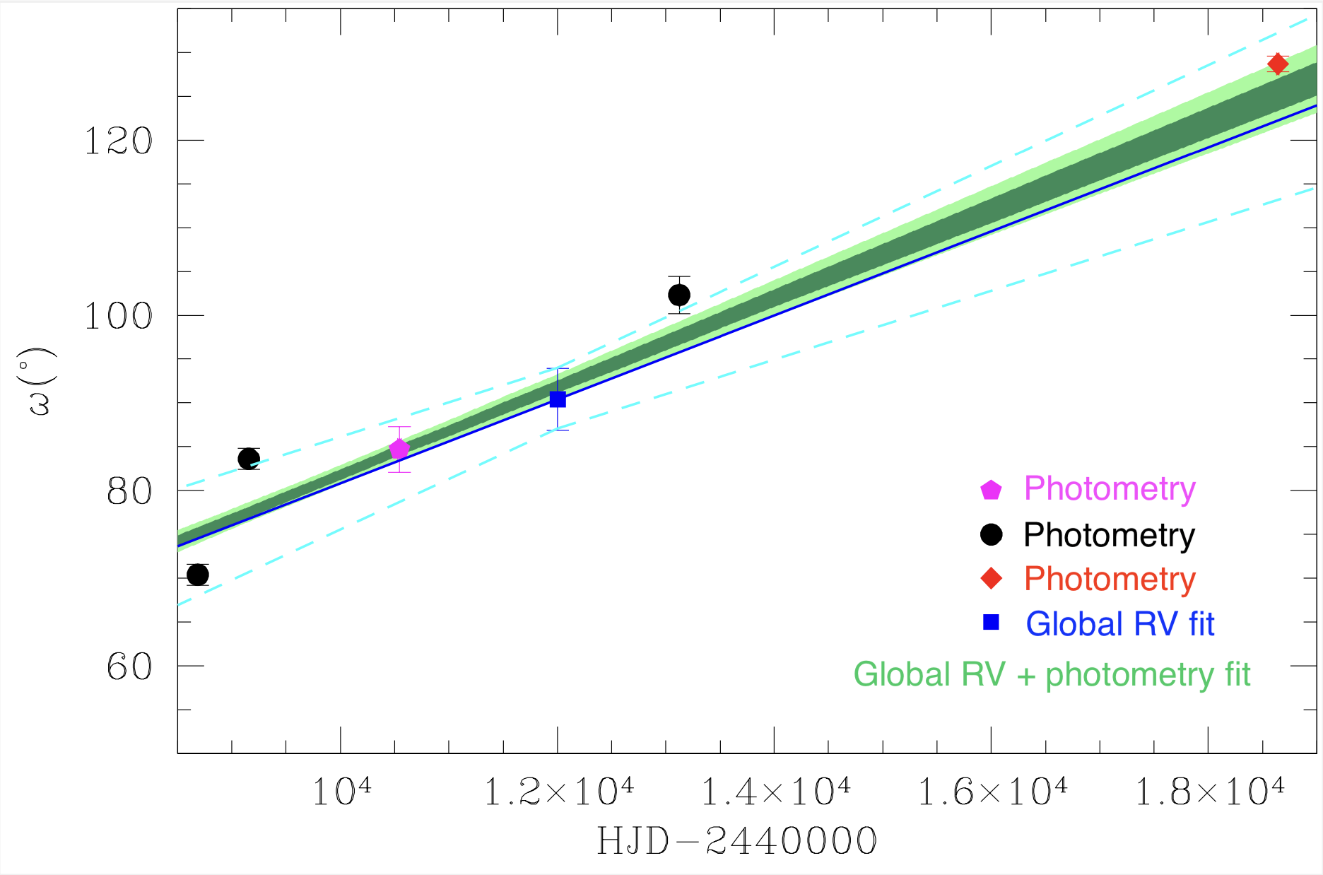
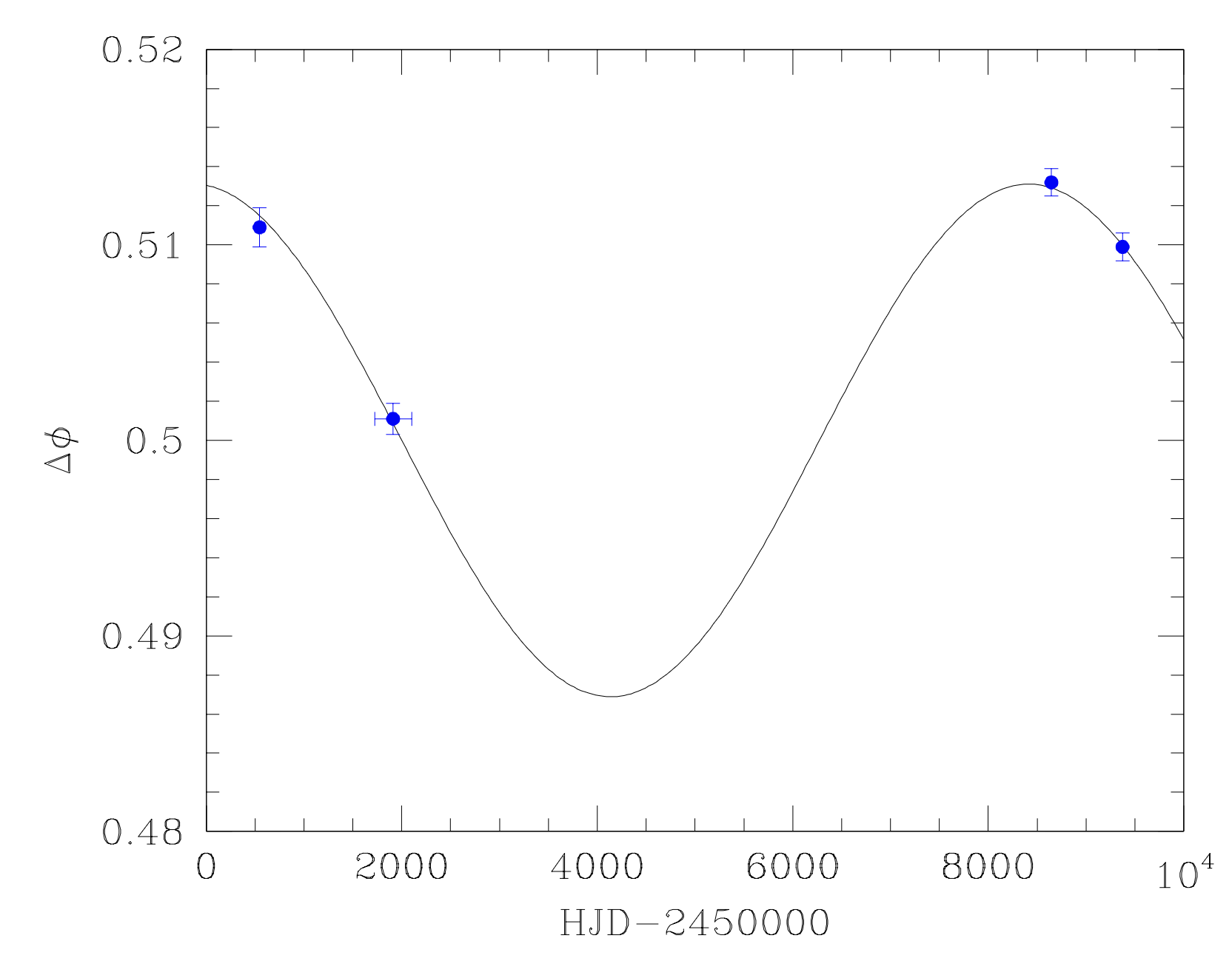
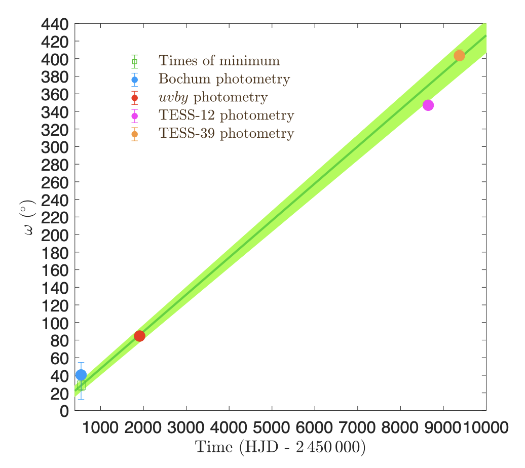
- Slow precession of the line of apsides in an eccentric binary;
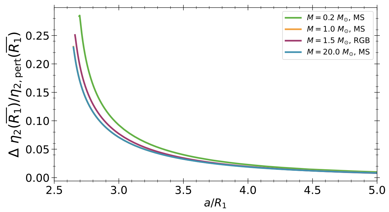
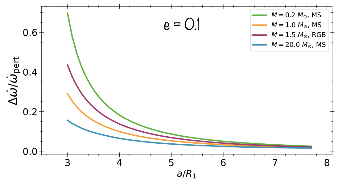
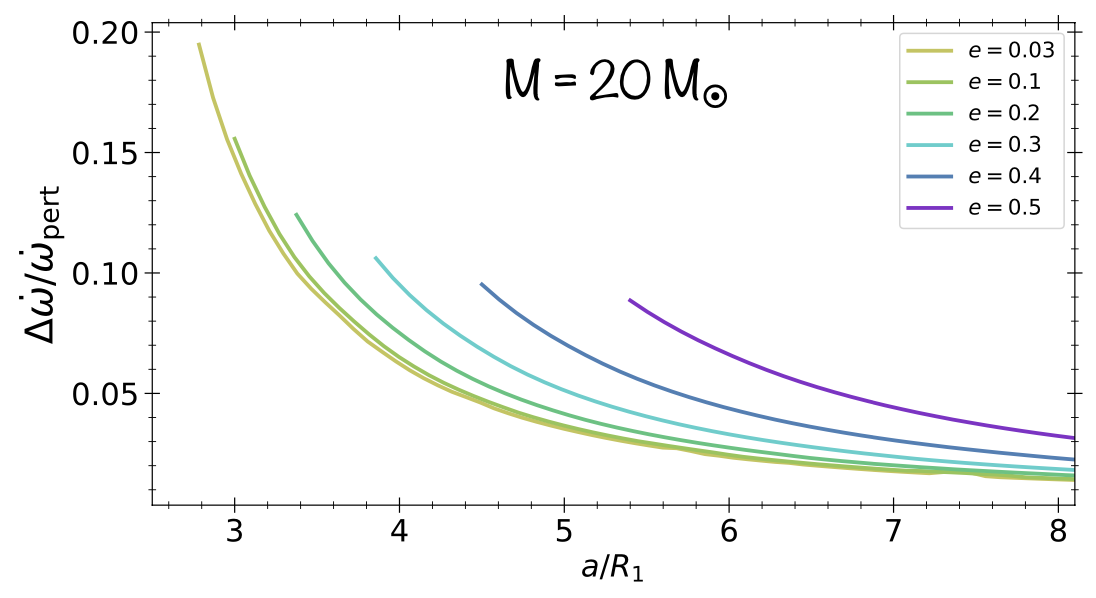
- Arises from tidal interactions occurring between the stars of a close binary, interactions which are responsible for the non-spherical gravitational field of the stars;
- Non-Keplerian movement (with a general relativistic contribution but small in the cases we study here).
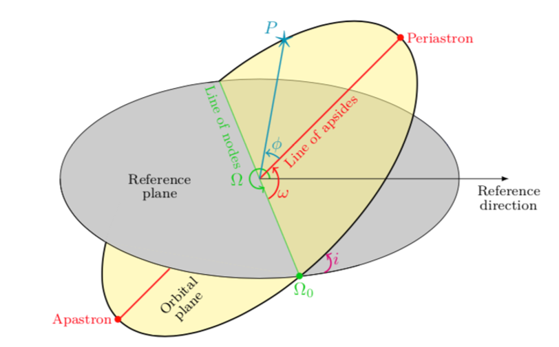
Definition of the orbital elements.
Artistic exaggerated illustration of the apsidal motion.
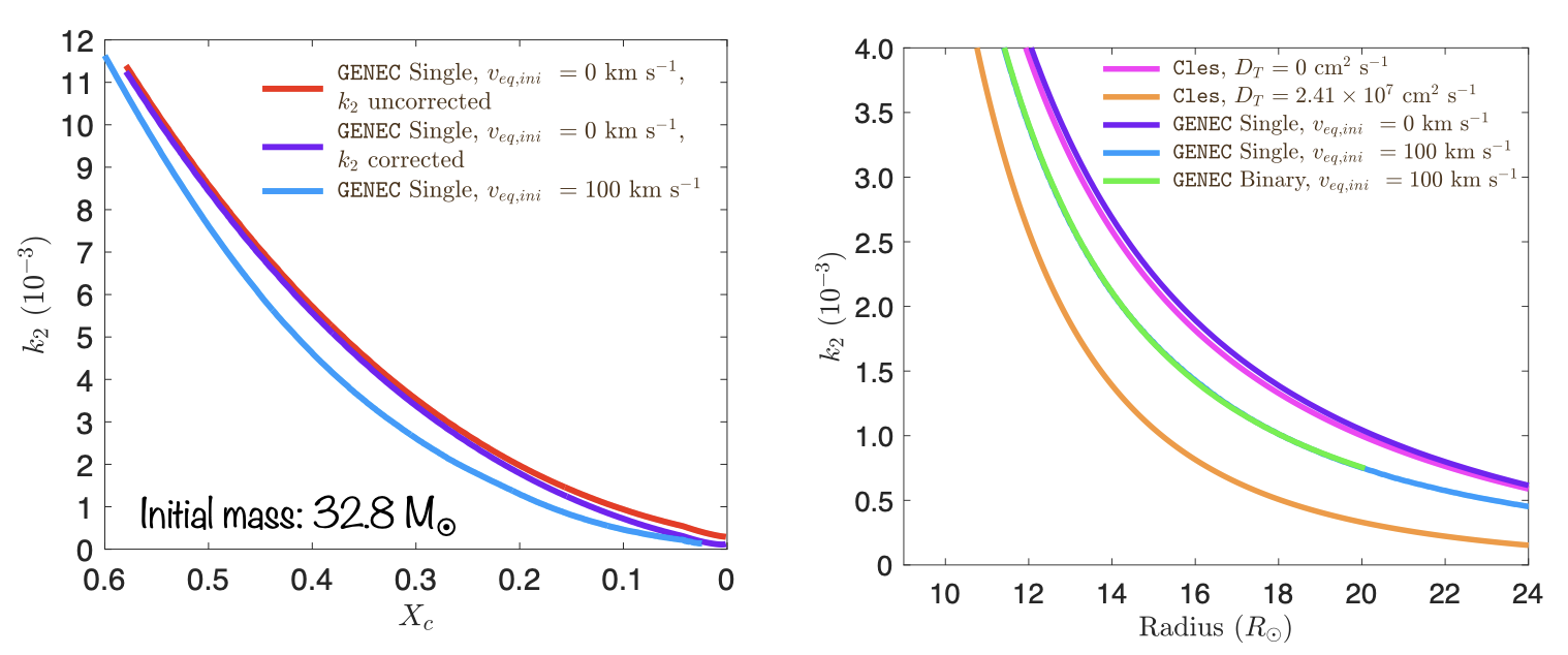
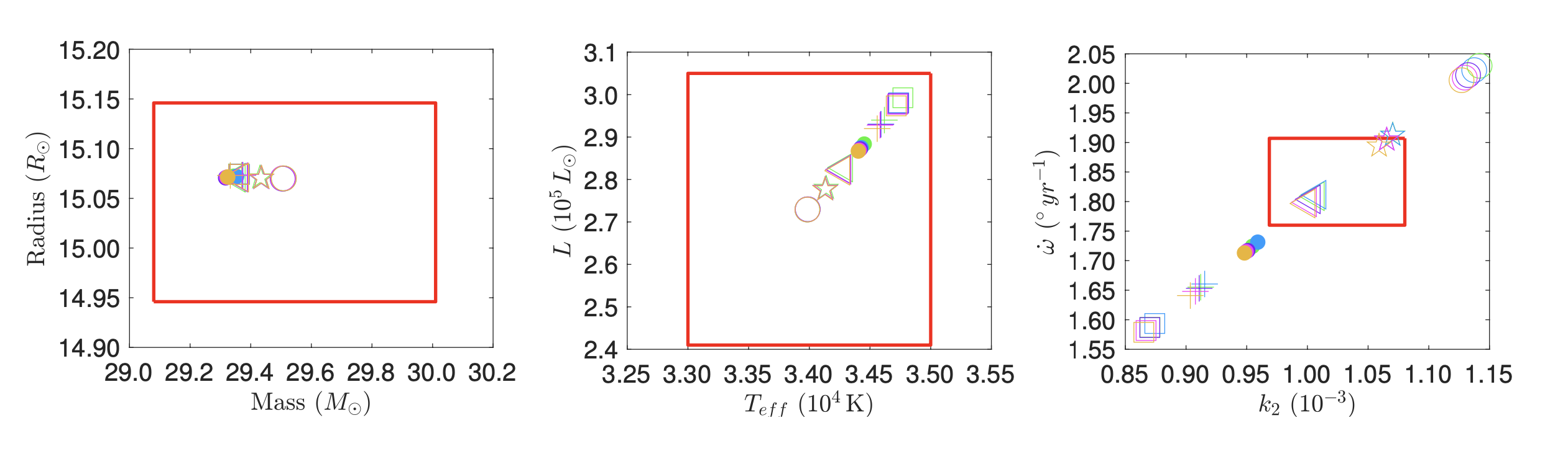
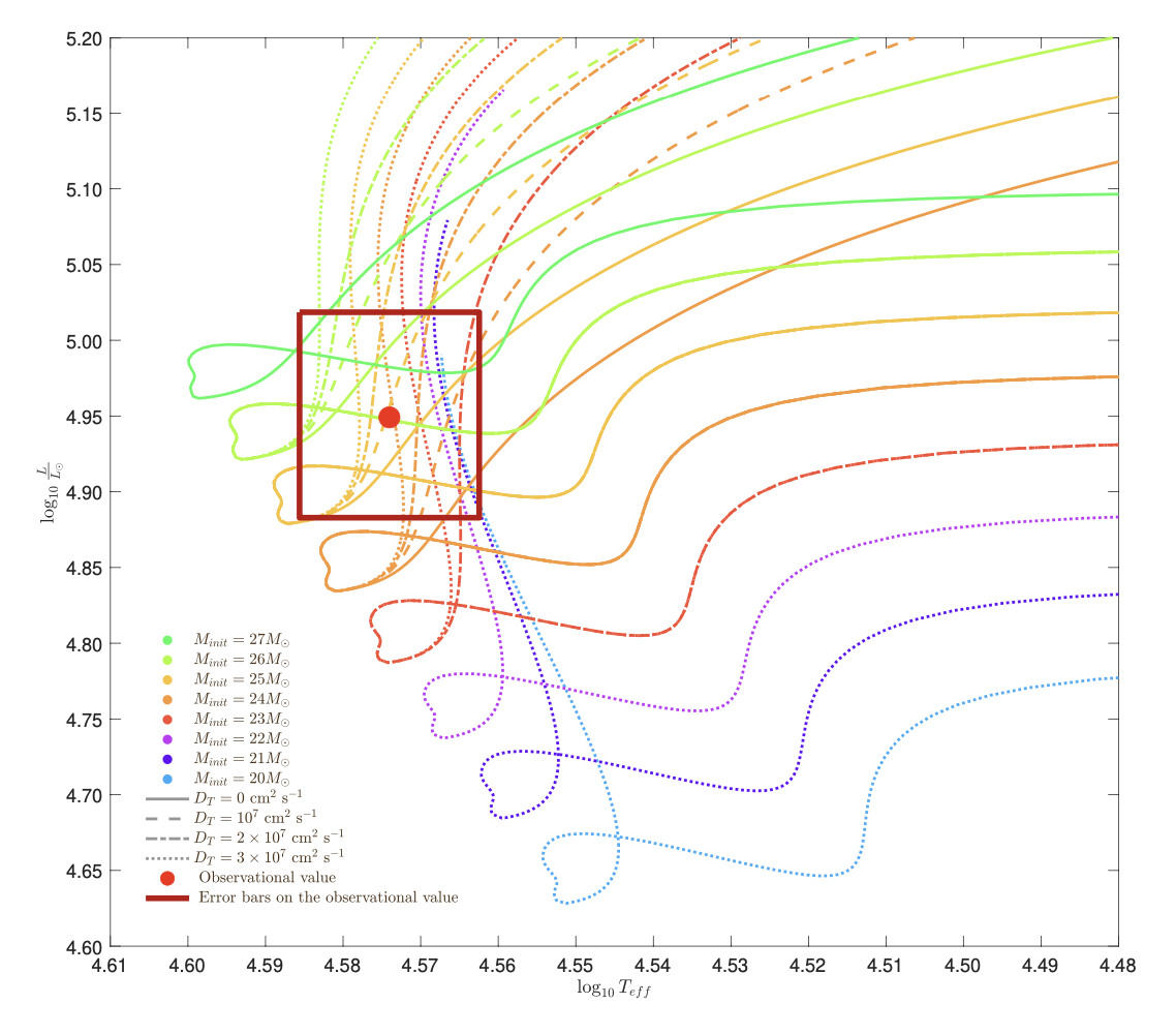
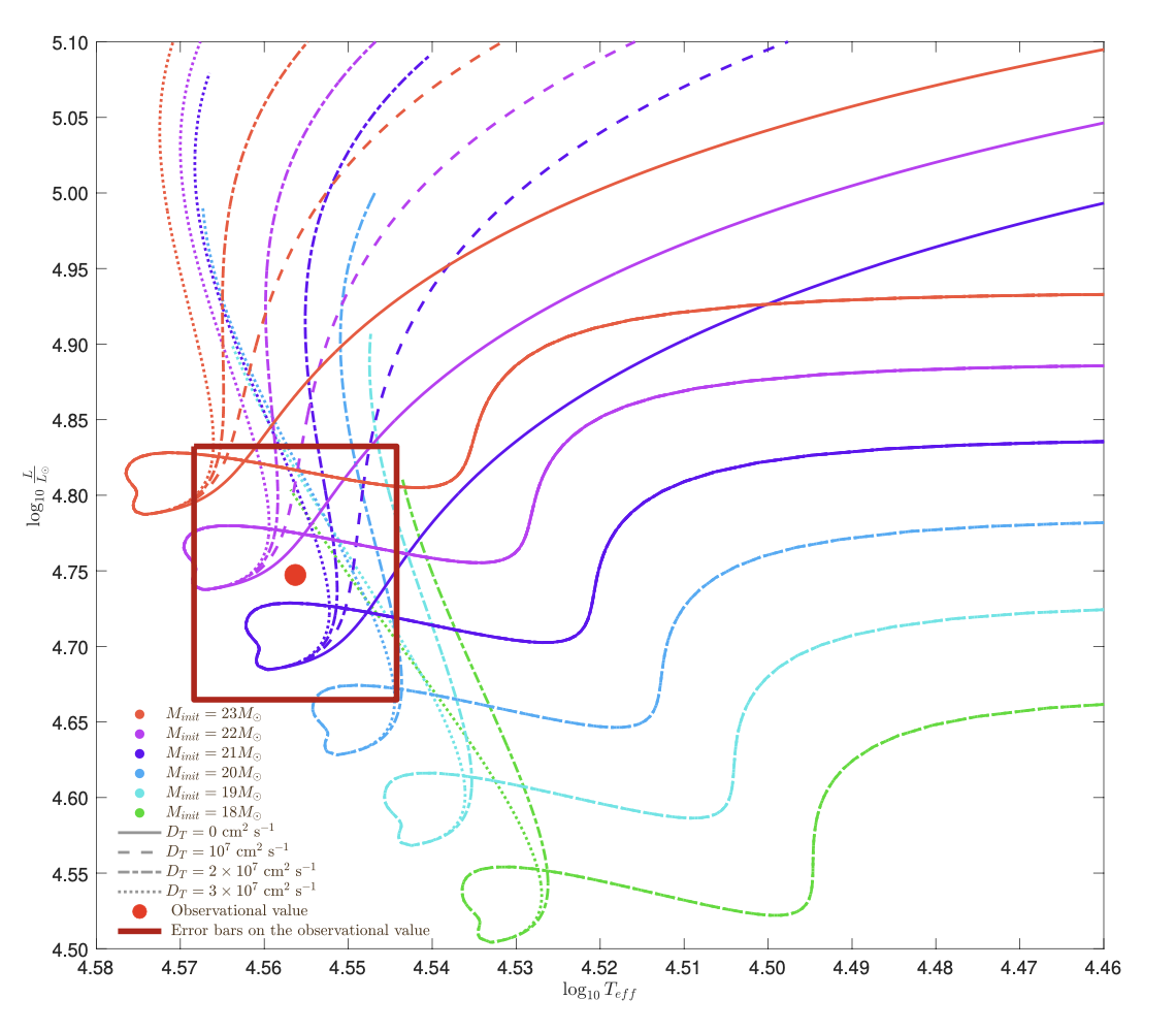
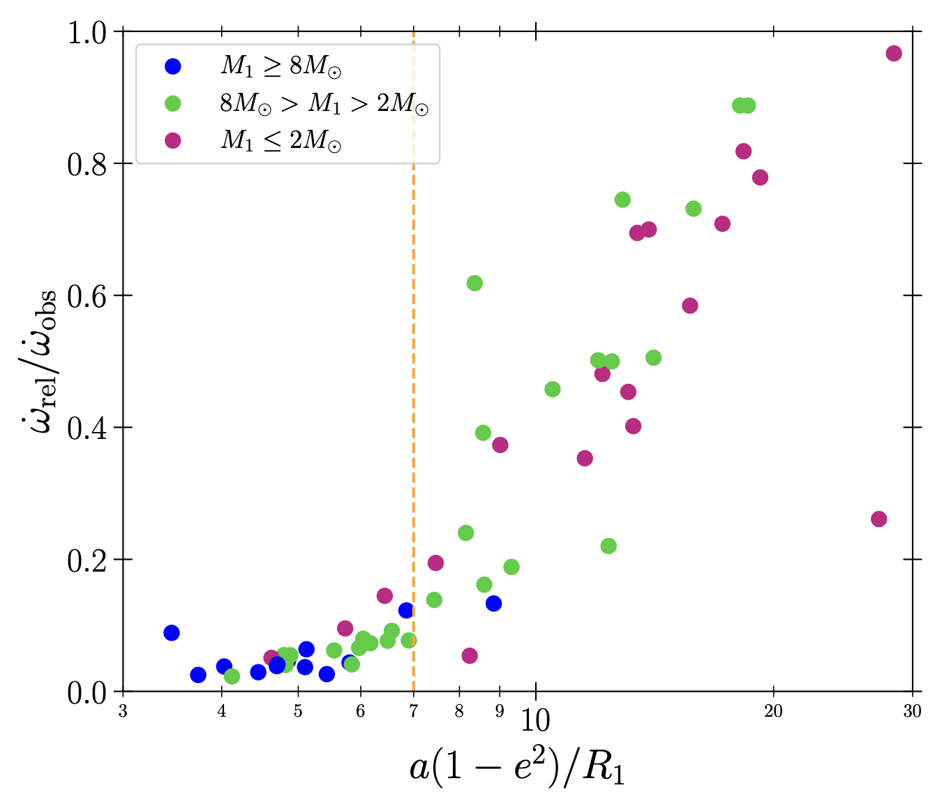
- The rate of apsidal motion is directly related to the internal structure of the stars. Measuring the rate of apsidal motion hence
- Provides a diagnostic of the internal mass-distribution of the stars, which is otherwise difficult to constrain;
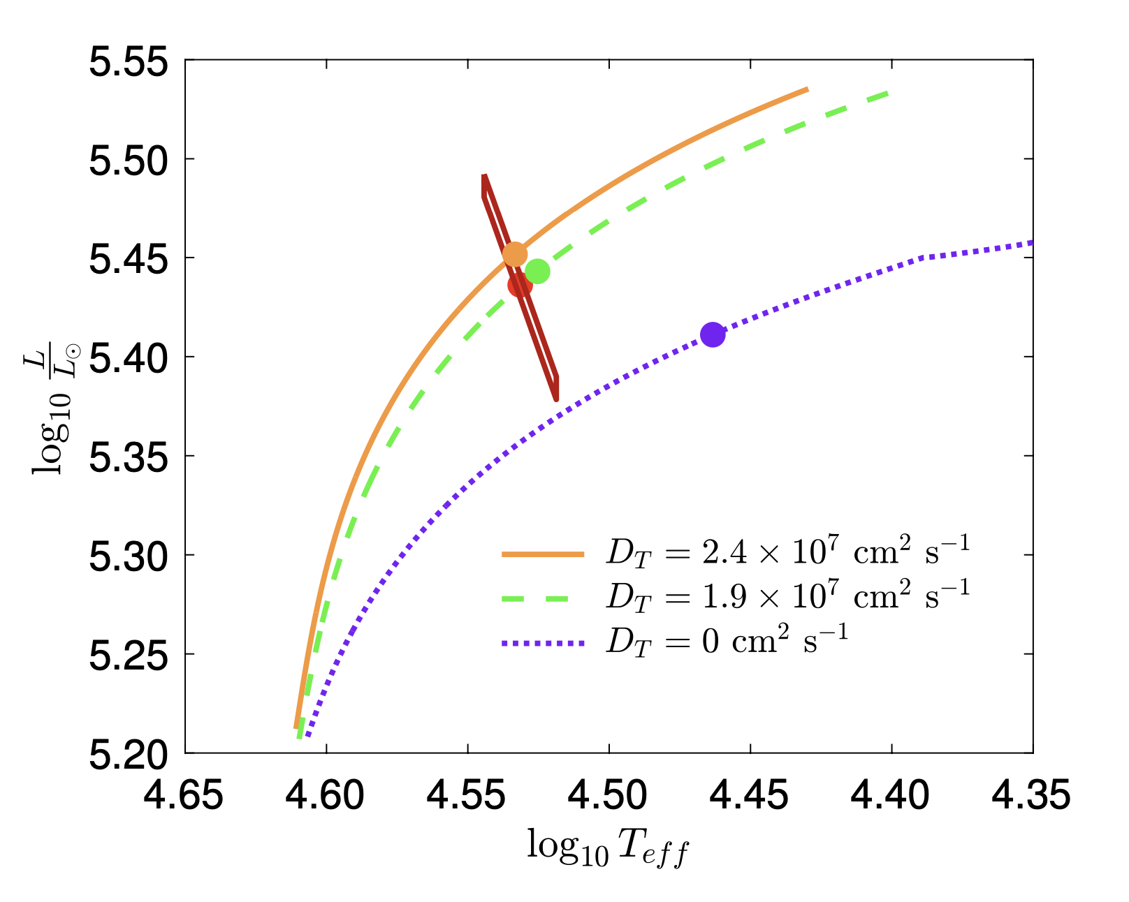
- Offers a test of our understanding of stellar structure and evolution.
In summary, if we want to constrain the internal structure of stars, we should study the apsidal motion in (massive) eccentric binaries!
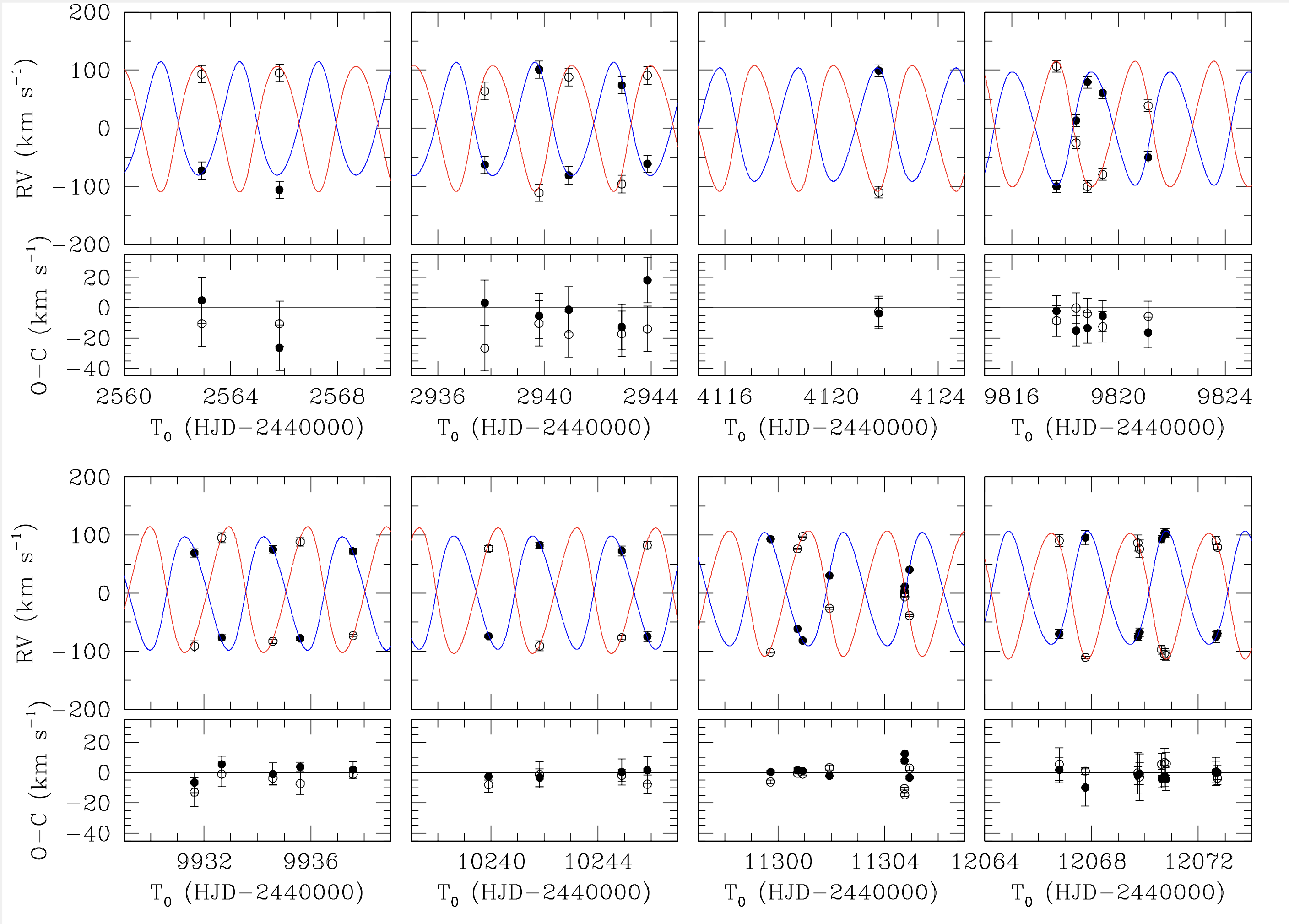
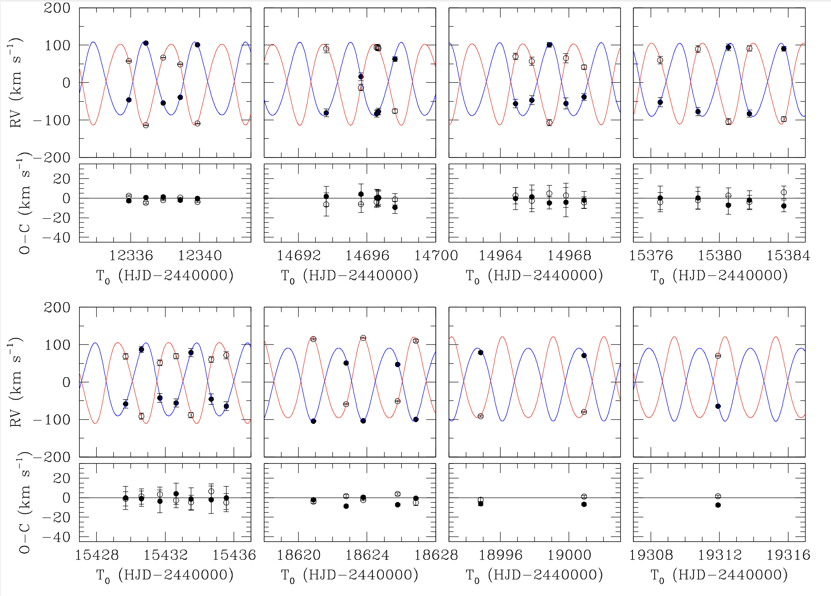
Is the apsidal motion observed and measured? YES!
The apsidal motion has been derived in hundreds of systems. Here, we report two large-scale studies (left and middle panels) as well as individual studies each focused on one single system (right panel).
Milky Way, LMC, and SMC binaries (Hong et al. 2016, MNRAS, 460, 650)
162 binaries in the LMC (Zasche et al. 2020, A&A, 640, A33)
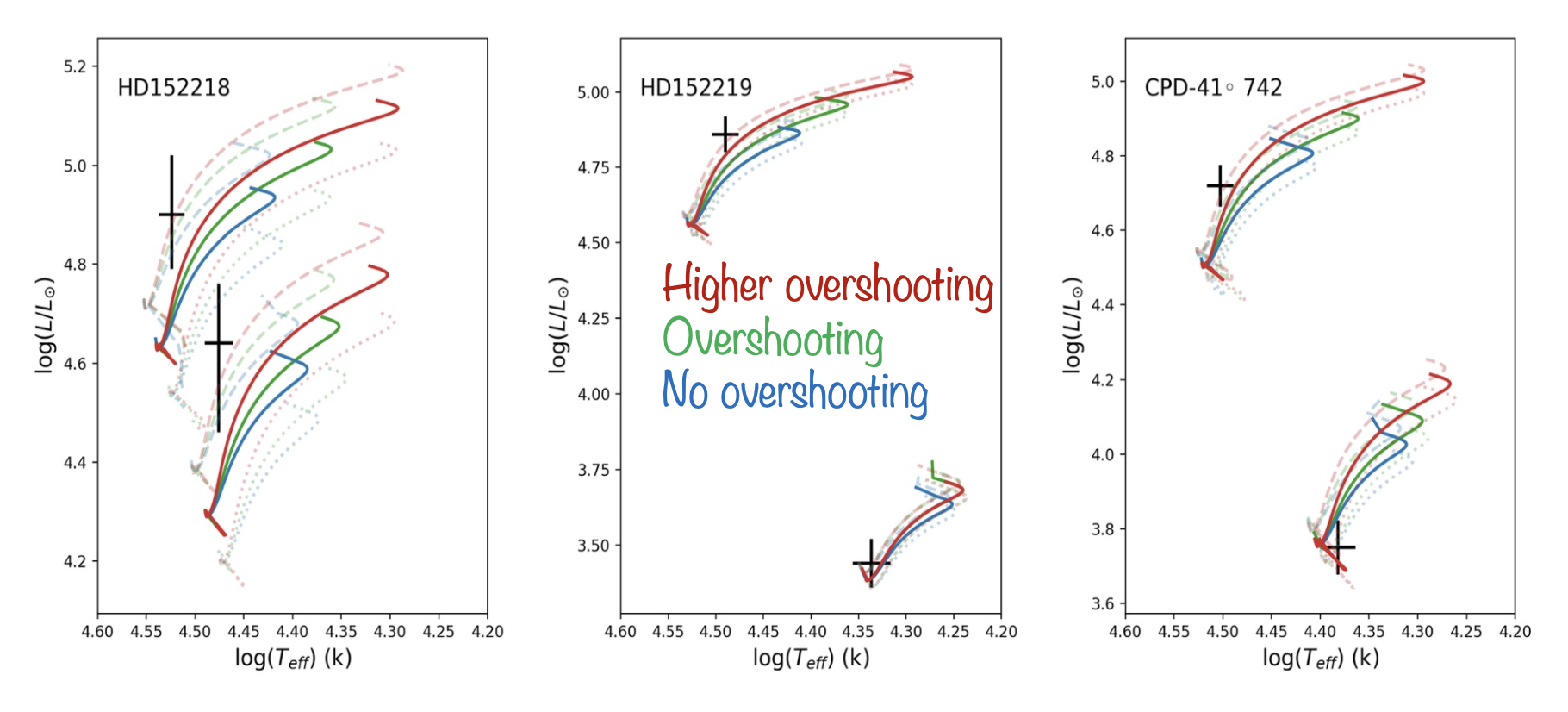
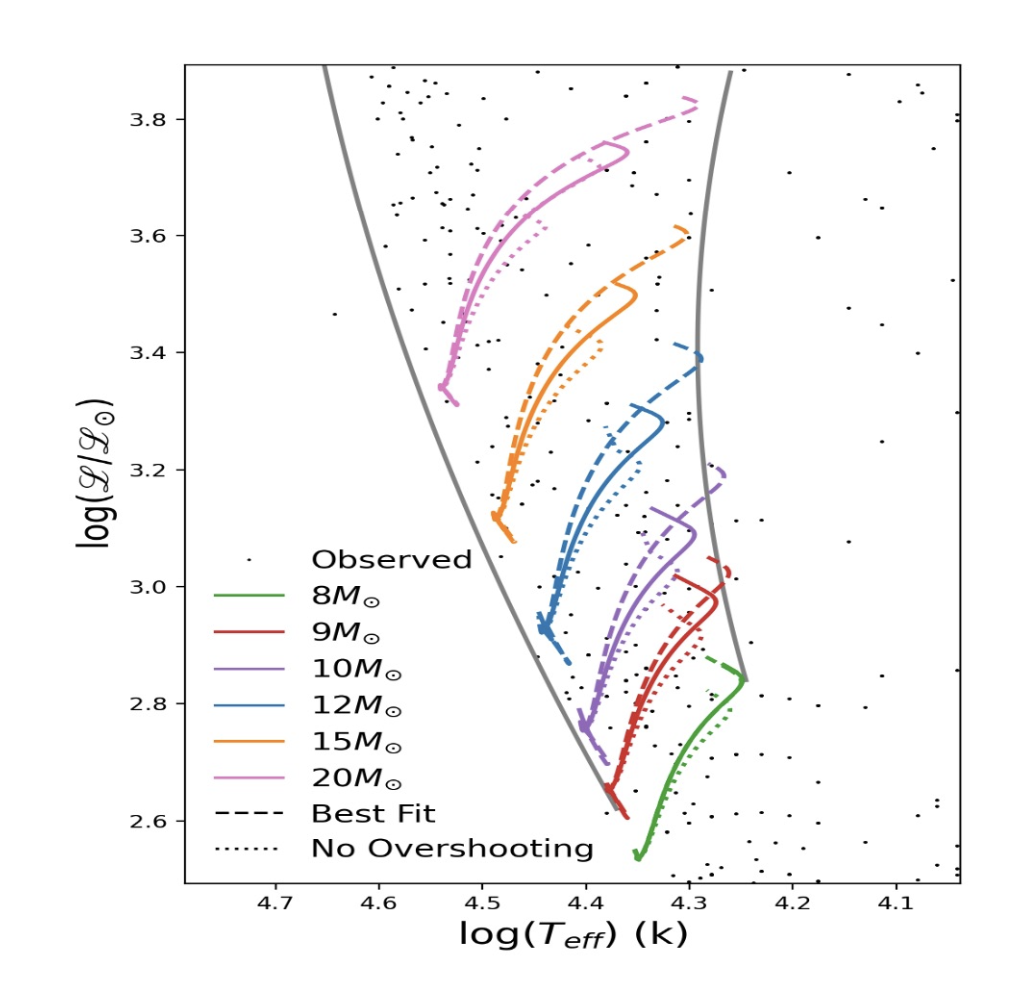
Individual studies of binaries (Rosu et al. 2023, CEAB, in press)
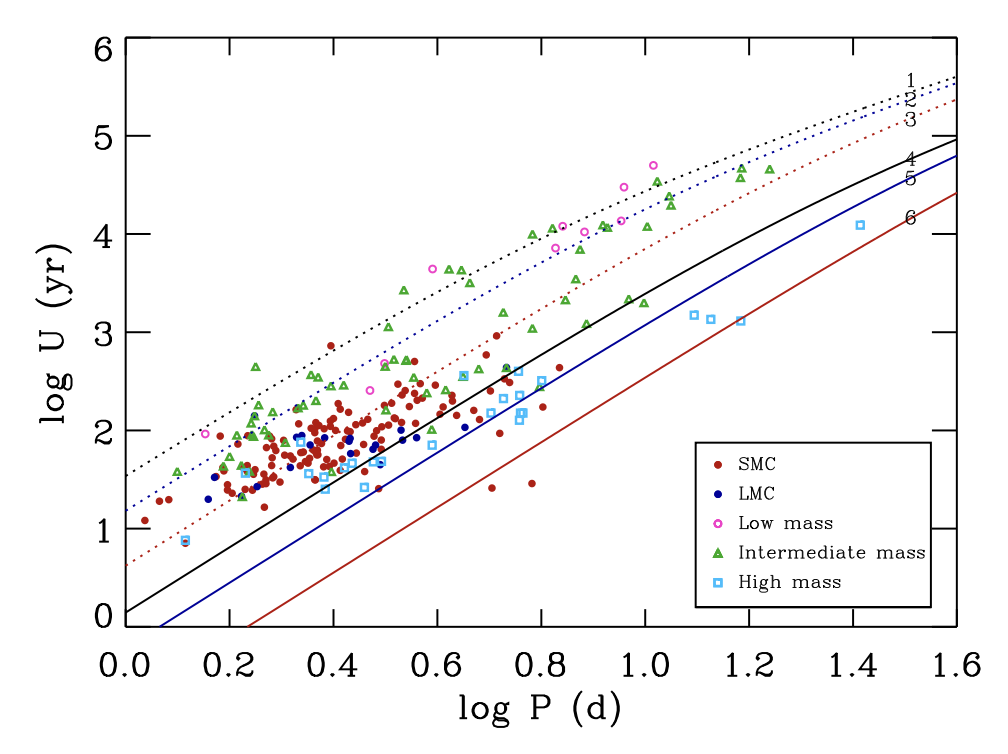
Apsidal motion period as a function of the orbital period of the system.
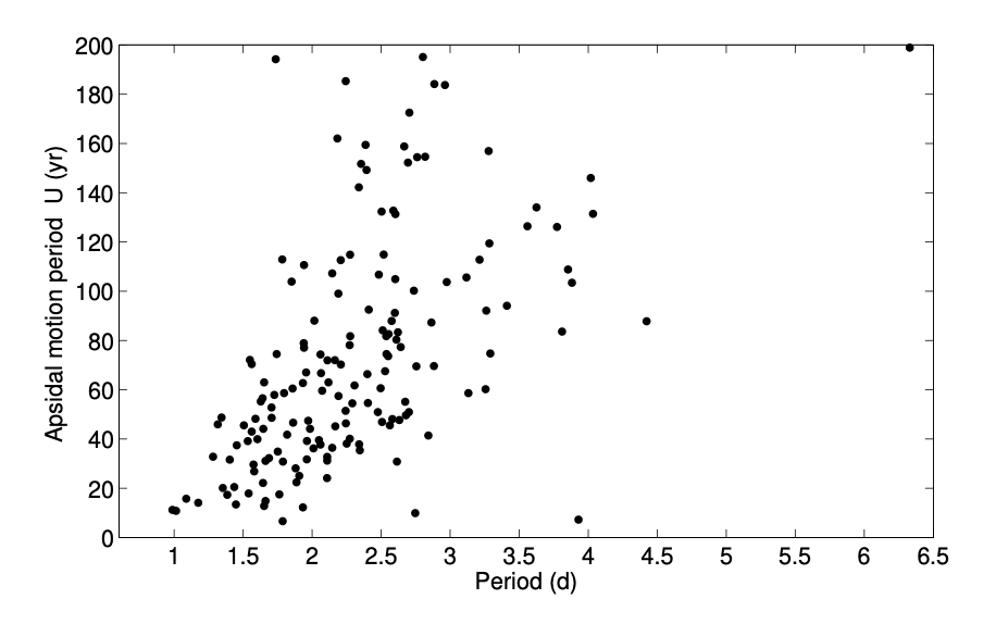
Apsidal motion period as a function of the orbital period of the system.
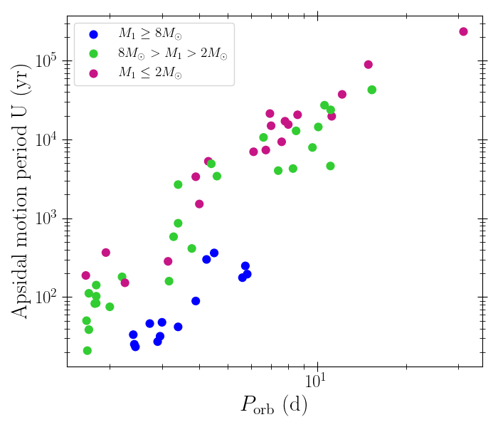
Apsidal motion period as a function of the orbital period of the system. Only primary stars are depicted.
Right panel: data from Baroch et al. 2021, A&A, 649, A64; Baroch et al. 2022, A&A, 665, A13; Claret et al. 2021, A&A, 654, A17; Marcussen & Albrecht 2022, ApJ, 933, 227; Rauw et al. 2016, A&A, 594, A33; Rosu et al. 2020, A&A, 635, A145; Rosu et al. 2022, A&A, 660, A120; Rosu et al. 2022, A&A, 664, A98; Rosu et al. 2023, MNRAS, 521, 2988; Torres et al. 2010, A&A Rev., 18, 67; Wolf et al. 2006, A&A, 456, 1077; Wolf et al. 2008, MNRAS, 388, 1836; Wolf et al. 2010, A&A, 509, A18).