Physical and chemical structure of the Serpens filament: fast formation and gravity-driven accretion

Yan Gong ¹ , Arnaud Belloche ¹ , Fujun Du ² , Karl Menten ¹ , Christian Henkel ¹ , Guangxing Li ³ , Friedrich Wyrowski ¹ , Ruiqing Mao ²

Abstract

The Serpens filament, a prominent elongated structure in a relatively nearby molecular cloud, is believed to be at an early evolutionary stage, so studying its physical and chemical properties can shed light on filament formation and early evolution. We performed 13CO (1–0), C18O (1–0), C17O (1–0), 13CO (2–1), C18O (2–1), and C17O (2–1) imaging observations toward
the Serpens filament with the IRAM-30m and APEX telescopes to address the physical and chemical properties as well as the dynamical state of the Serpens filament at a spatial resolution of ∼0.07 pc and a spectral resolution of ~0.1 km/s. Widespread narrow 13CO (2–1) self-absorption is observed in this filament, causing the 13CO morphology to be different
from the filamentary structure traced by C18O and C17O. Our excitation analysis suggests that the opacities of C18O transitions become
higher than unity in most regions, and this analysis confirms the presence of widespread CO depletion. Further we show that the local
velocity gradients have a tendency to be perpendicular to the filament’s long axis in the outskirts and parallel to the large-scale
magnetic field direction. The magnitudes of the local velocity gradients decrease toward the filament’s crest. The observed velocity
structure can be a result of gravity-driven accretion flows. The isochronic evolutionary track of the C18O freeze-out process indicates
the filament is young with an age of ≤2 Myr. We propose that the Serpens filament is a newly-formed slightly-supercritical structure which appears to be actively accreting material from its ambient gas.

1. Initial collapse

One of the nearest infrared dark clouds

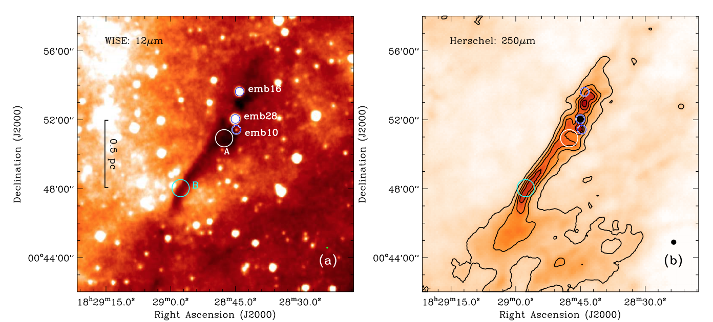
Figure 1: (a) WISE 11.2 μm image of the Serpens filament that shows up in absorption. (b) Herschel 250 μm image of the Serpens filament seen in emission.

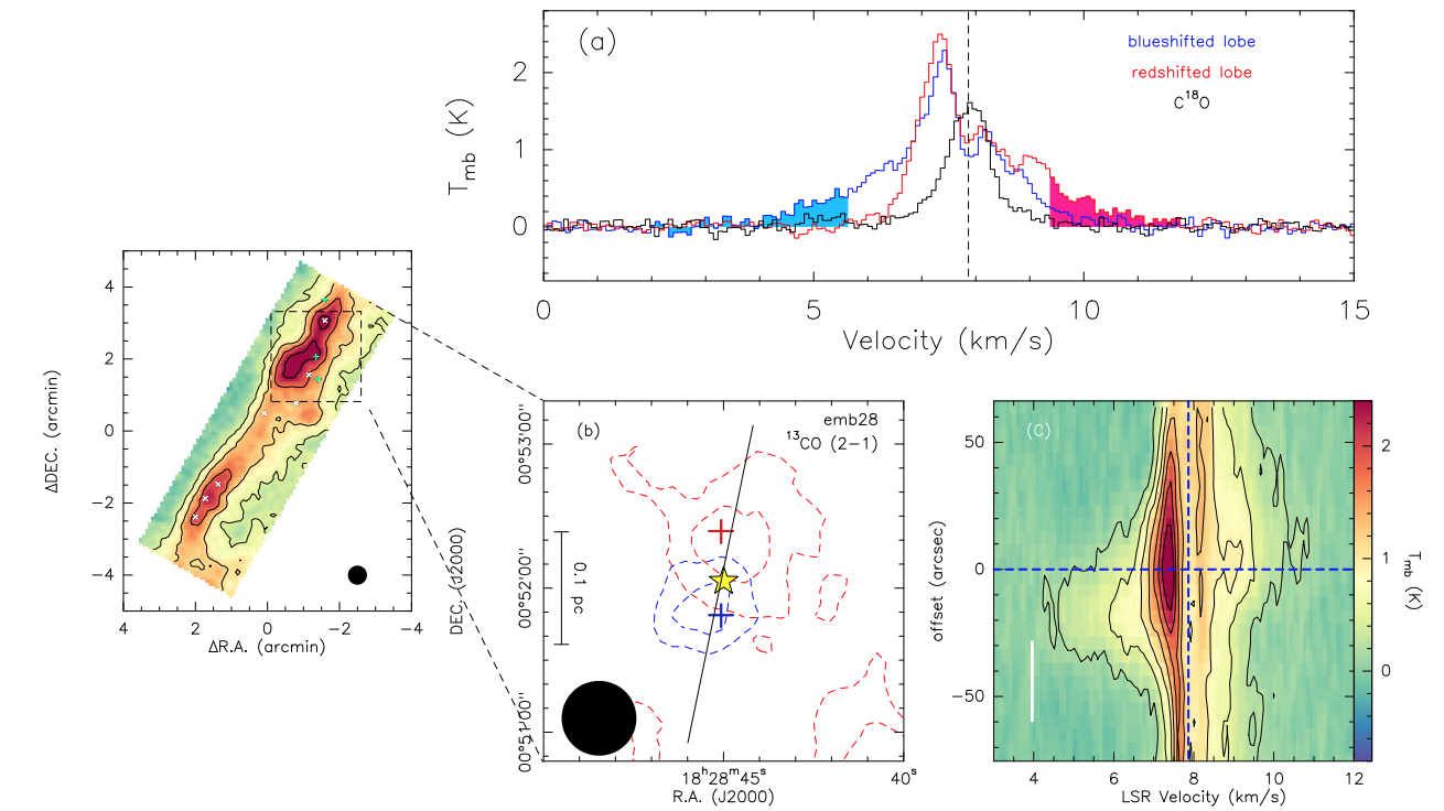
Widespread blue-skewed emission

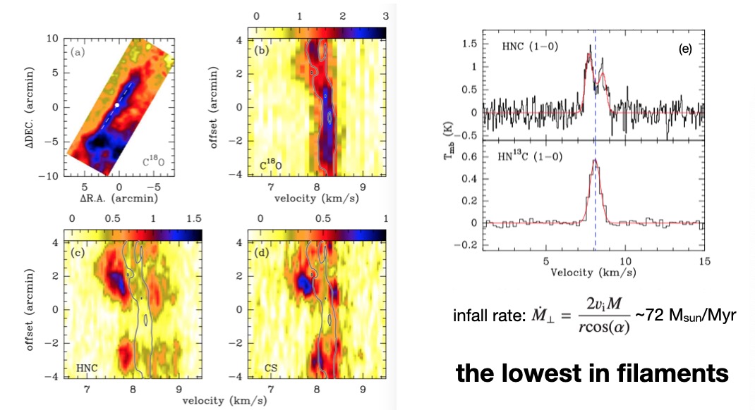
Figure 2 (a) C¹⁸O (1–0) integrated intensity map overlaid with a PV cut indicated by the white dashed line. (b): PV diagram of C¹⁸O (1–0) along the PV cut in panel a. (c): similar to panel b but for HNC (1–0). Panel d: similar to panel b but for CS (2–1). In panels b–d, the color bars represent main beam brightness temperatures in units of K, and the black contours represent the C¹⁸O (1–0) emission starting at 1.5 K (5σ) with increments of 0.9 K (3σ). (e) Observed line profiles of HNC (1-0) and HN¹³C (1-0).

Gong, Y., Li, G. X., Mao, R. Q., Henkel, C., Menten, K. M., Wang, M., Sun, J. X. et al. 2018, A&A, 620, A62

00:00 --:--

2. Molecular analysis

Overall molecular distribution

Figure 3: Integrated intensity maps of ¹³CO (1–0) (a), C¹⁸O (1–0) (b), C¹⁷O (1–0) (c), ¹³CO (2–1) (d), C¹⁸O (2–1) (e), and C¹⁷O (2–1) (f).

The morphology of the emission of the two ¹³CO lines is markedly different because of significant ¹³CO self-absorption.

Discovery of a new molecular outflow driven by Ser-emb 28

Figure 4: Outflow driven by Ser-emb 28. Left: Same as Fig. 4e. Right: (a) Observed ¹³CO (2–1) spectra of the two positions indicated by the blue and red pluses in panel (b) overlaid with the C¹⁸O spectrum of the position indicated by the yellow star in panel (b). (b) ¹³CO (2–1) outflow map of Ser-emb 28. The yellow star marks the position of Ser-emb 28. The beam size is shown in the lower left corner. (c) Position-velocity diagram of the ¹³CO (2–1) emission along the cut indicated by the black line in panel b.

LTE analysis with MCMC calculations

Figure 5: Posterior probability distributions of C¹⁸O column density, N_C18O, rotational temperature, Trot, the C¹⁸O (1–0) opacity, τ_18,1, and the C¹⁸O (2–1) opacity, τ_18,2, toward the dense core, Bolo12, with the maximum posterior possibility point in the parameter space shown in orange lines and points. Contours denote the 0.5σ, 1.0σ, 1.5σ, and 2.0σ confidence intervals.

This analysis suggests that the opacities of C¹⁸O (1–0) and C¹⁸O (2–1) become higher than unity in most regions.

Rotational temperature, column density and molecular abundance

Figure 6: (a) C¹⁸O rotational temperature map. (b) C¹⁸O column density map. (c) C¹⁸O fractional abundance map overlaid with H₂ column density contours.

This result has confirmed the presence of widespread CO depletion.

Gong, Y., Belloche, A., Du, F. J., Menten, K. M., Henkel, C., Li, G, X., Wyrowski, F., Mao, R. Q. 2021, A&A, 646, A170

00:00 --:--

4. Chemical timescale

The chemical isochronic evolutionary track

Figure 10: (a): C¹⁸O fractional abundances as a function of time, as calculated with Chempl (Du 2021) by adopting different H₂ column densities and an assumed thickness of 0.68 pc. (b): Observed C¹⁸O fractional abundance as a function of H₂ column density.

The isochronic evolutionary tracks of the C¹⁸O freeze-out process are indicated by the black lines. This novel method indicates that the filament is young with an age of ≲2 Myr.

Gong, Y., Belloche, A., Du, F. J., Menten, K. M., Henkel, C., Li, G, X., Wyrowski, F., Mao, R. Q., 2021, A&A, 646, A170

00:00 --:--

3. Accretion flows

Local velocity gradients

Figure 7: (a) Local velocity gradient magnitude map overlaid with H₂ column density contours. (b) Herschel H₂ column density map overlaid with the normalized velocity vector maps. The arrows represent the estimated local velocity gradients which are rotated by 180° in order to better visualize the accretion directions in SE. The polarized angle of the Planck 353 GHz thermal dust emission has been rotated by 90° to trace the magnetic field direction which is indicated by the red line. The three green pluses give the positions of the three embedded YSOs, emb10, emb16, and Ser-emb 28 (Enoch et al. 2009), and the white crosses mark the positions of the seven dust cores (Enoch et al. 2007).

We show that the local velocity gradients have a tendency to be perpendicular to the filament's long axis in the outskirts and parallel to the large-scale magnetic field direction. The magnitudes of the local velocity gradients decrease toward the filament's crest. The observed velocity structure can be a result of gravity-driven accretion flows. The scenario is illustrated in Figs. 8 and 9. The vectors are also wrapping the filament’s southern end, consistent with the predictions for the edge effect of a finite filament.

Figure 8: Schematic view of the geometry of the Serpens filament. The left panel gives a perspective view of its 3D geometry, and the right panels represent the projection on to the x-y, x-z, and y-z planes. The midplane and its parallel surfaces have the same distances to observers, and the line of sight is along the z direction. The local velocity gradients that are associated with blueshifted and redshifted flows are indicated by the blue and red arrows, while the magnetic field is indicated by green dashed lines.

Figure 9: Schematic animation of the kinematics of the Serpens filament

Gong, Y., Belloche, A., Du, F. J., Menten, K. M., Henkel, C., Li, G, X., Wyrowski, F., Mao, R. Q., 2021, A&A, 646, A170

00:00 --:--

1. Initial collapse

2. Molecular analysis

4. Chemical timescale

3. Accretion flows

5. 3D view