Applying machine-learning methods to build a photometric classifier for massive stars in nearby galaxies

• display strong stellar winds
• deposit energy and momentum to the interstellar medium
• produce a series of elements
• shed chemically processed material as they evolve
• enhance the galactic environment of their host galaxies when exploding as supernovae
• die as neutron stars or black holes, offering insights to extreme physics (gravity, temperature)
• are progenitors of gamma-ray bursts and gravitational wave sources
• are very luminous and can be observed in more distant galaxies > ideal tool to understand stellar evolution across cosmological time, especially for first galaxies (such as those to be observed with James Webb Space Telescope).

Key factors that determine their evolution:

• initial mass
• metallicity
• stellar rotation
• mass-loss
• binary interactions.

• affects strongly the stellar evolution
• enriches the immediate circumstellar environment
• forms complex structures (shells, disks, etc.).

Mass loss is not homogeneous, even at the simplest cases of stellar winds from single stars.

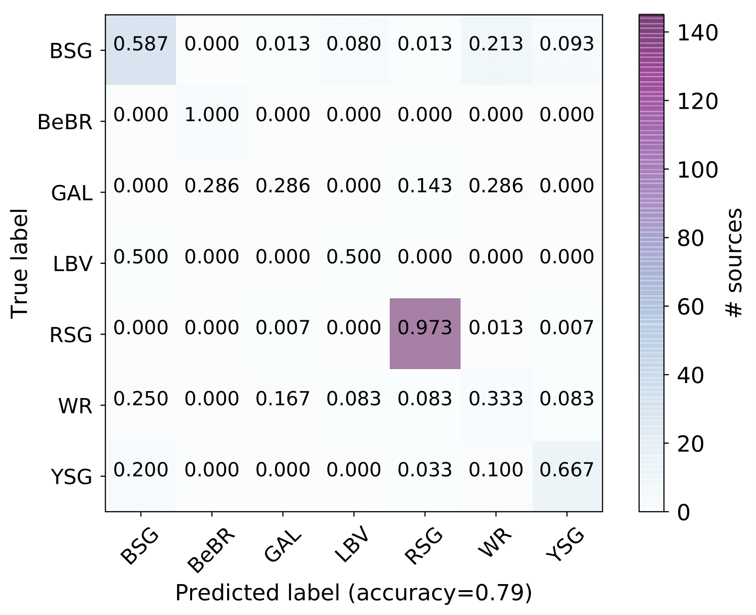
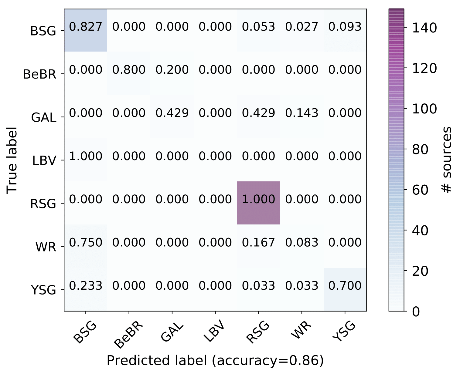
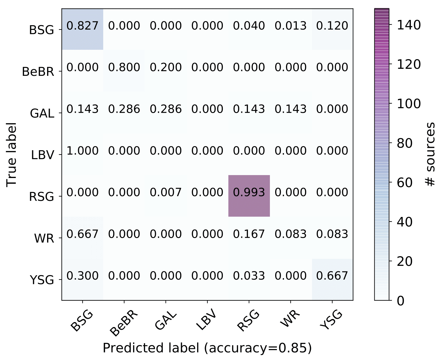
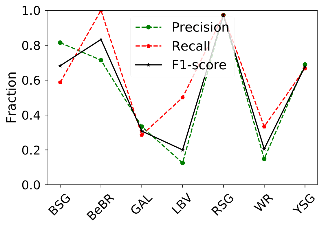
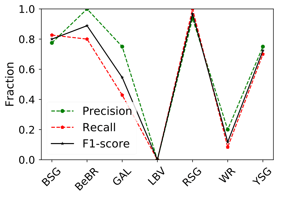
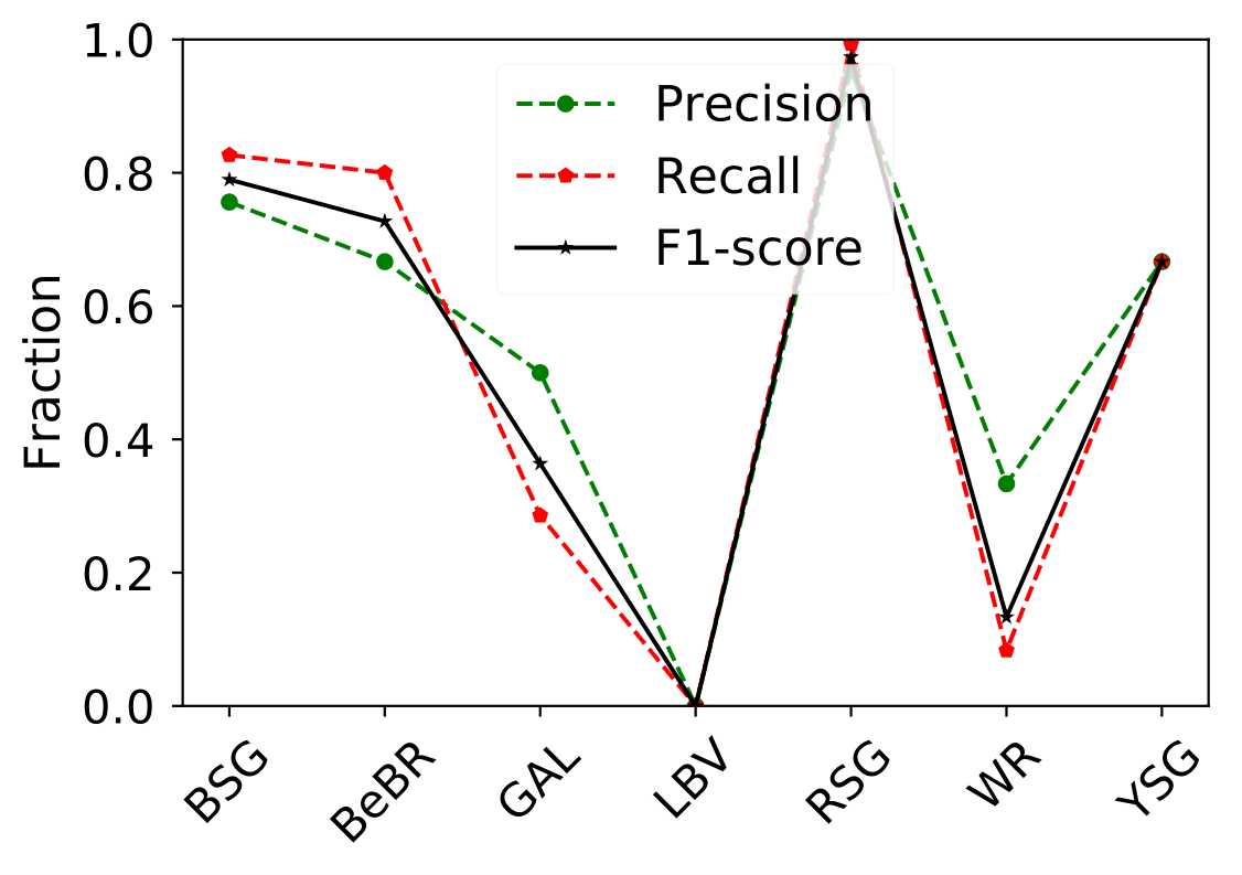
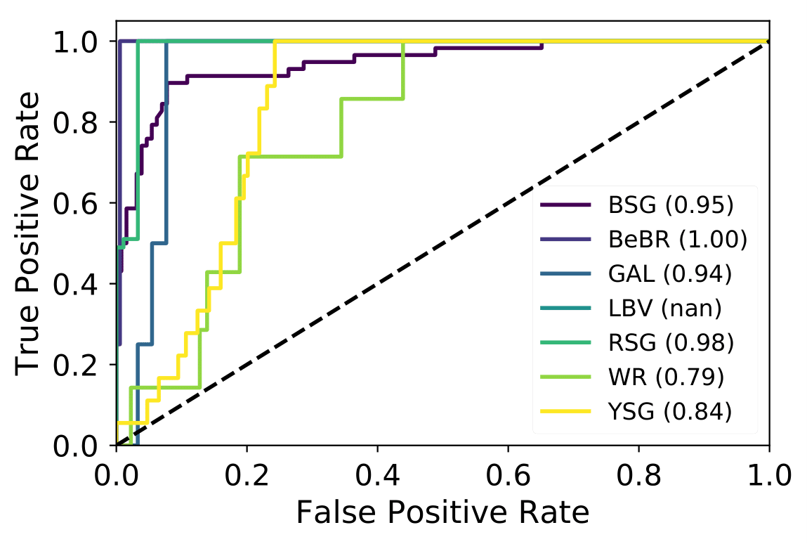
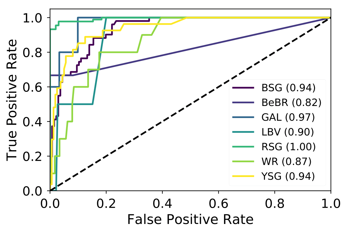
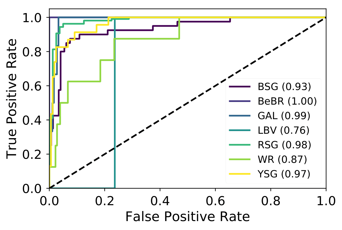
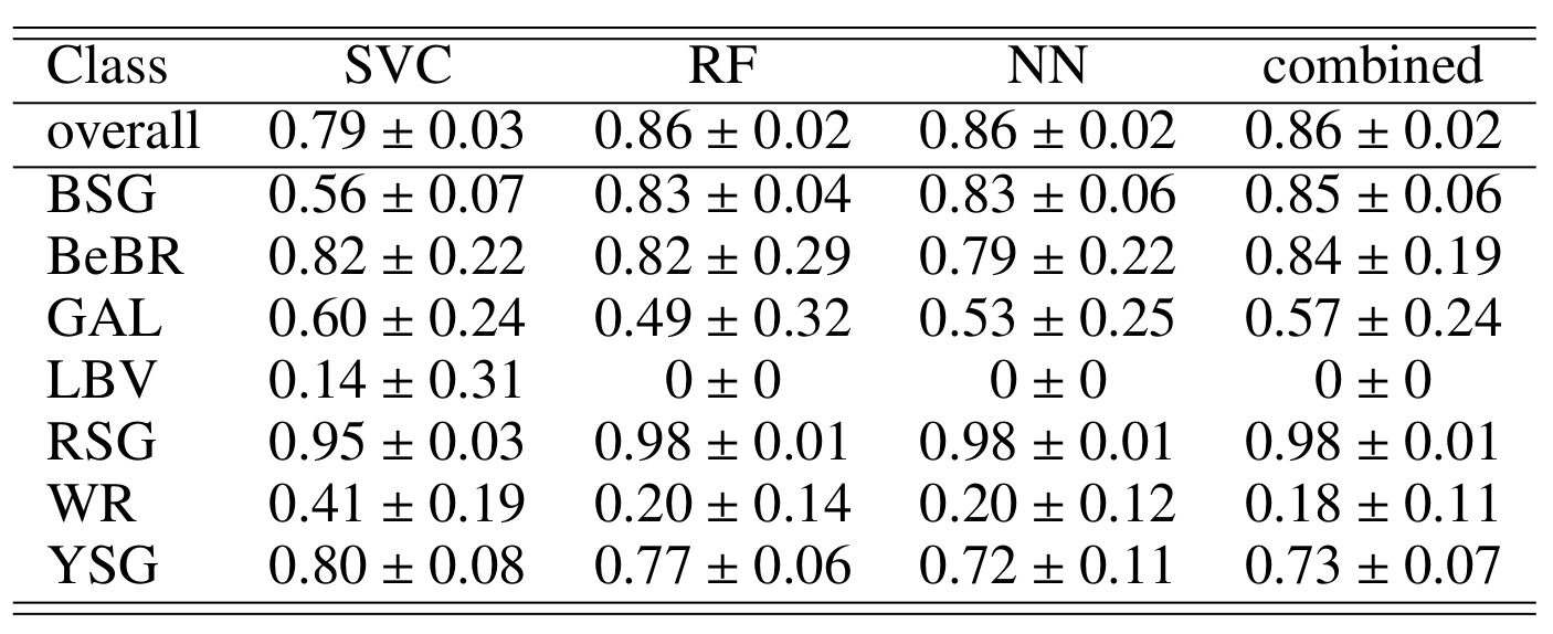
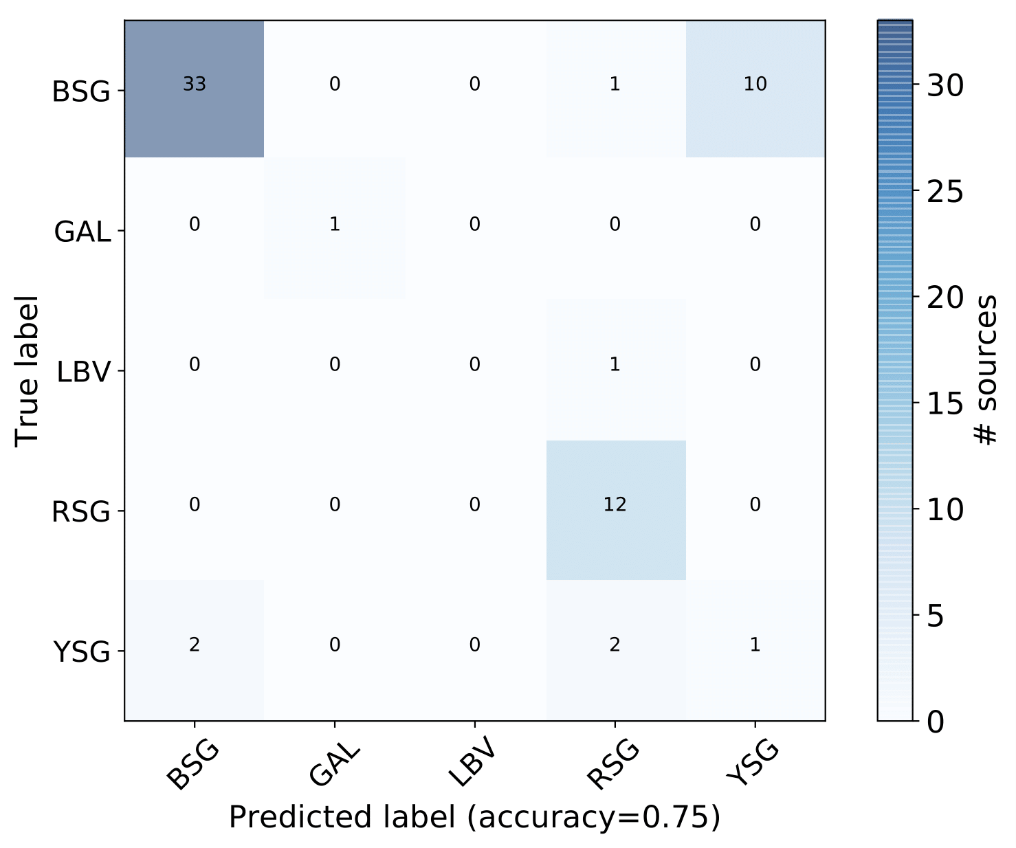
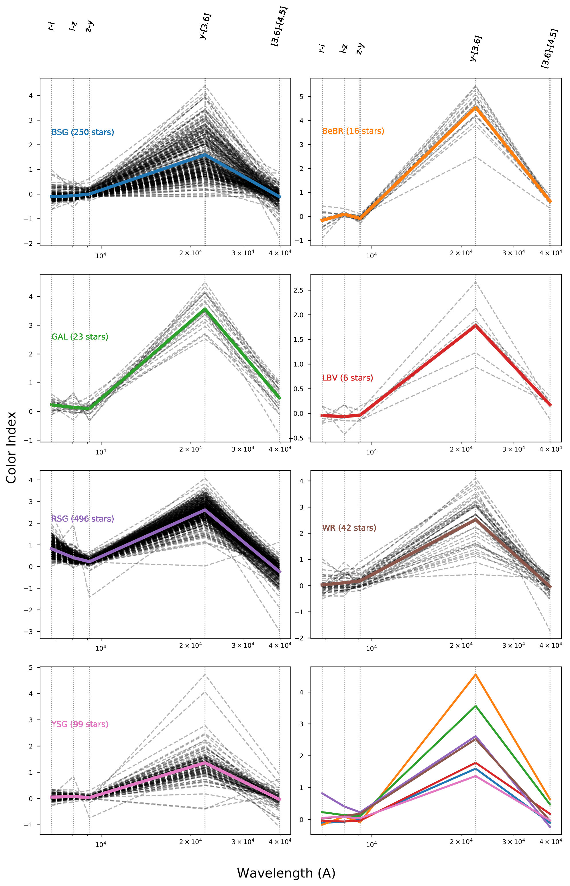
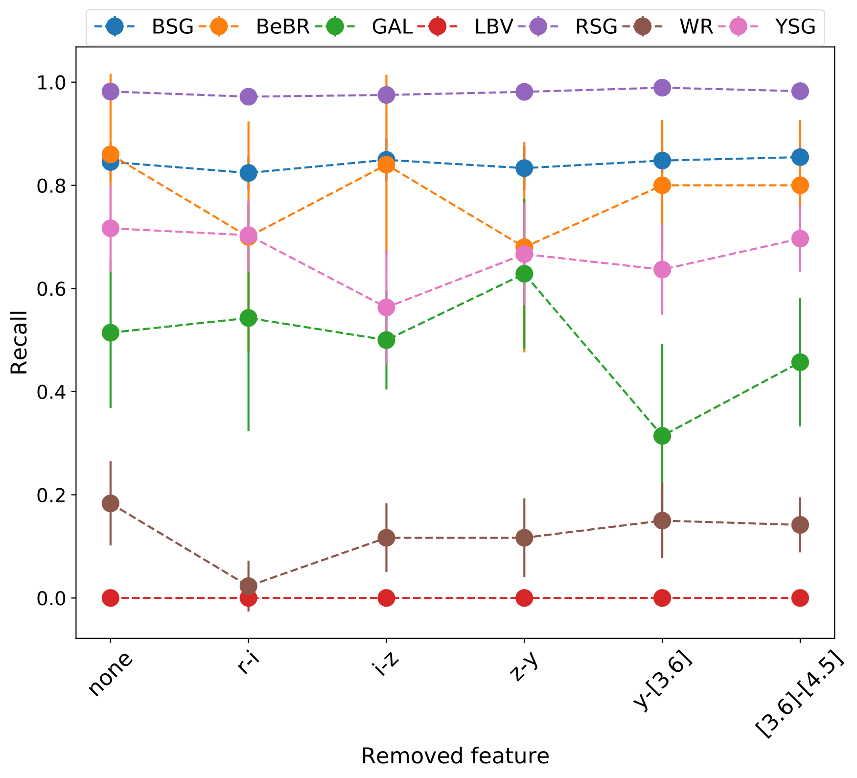
A number of massive stars experience episodic activity and outbursts, e.g. Wolf-Rayet stars (WR), Luminous Blue Variables (LBV), Blue Supergiants (BSG), B[e] Supergiants, Red Supergiants (RSGs), Yellow Supergiants (YSGs).

The presence of circumstellar material in various phases of massive stars and super luminous supernovae implies a central role of episodic mass loss in the evolution of massive stars. IR photometry is an ideal tool for distinguishing massive stars and in particular those with dusty environments (Bonanos et al. 2009, 2010, Britavskiy et al. 2014, 2015).

The ERC-funded project ASSESS  ("Episodic Mass Loss in Evolved Massive stars: Key to Understanding the Explosive Early Universe") aims to determine the role of episodic mass by:

• assembling a large sample of evolved massive stars in a selected number of nearby galaxies at a range of metallicities through multi-wavelength photometry,
• performing follow-up spectroscopic observations on candidates to validate their nature and extract stellar parameters,
• testing the observations against the assumptions and predictions of the stellar evolution models.

For the first step, we applied machine-learning techniques to mid-IR point-source catalogs from Spitzer Space Telescope that became publicly available only recently (Khan et al. 2015; Khan 2017; Williams & Bonanos 2016).

Upper panels: The confusion matrices for the SVC, RF, and NN methods, respectively.

Middle panels: The precision, recall, and f1-score metrics for SVC, RF, and NN methods, respectively. These results originate from single runs, i.e. by training each method with 70% of our sample and applying the classifier to the validation sample (30%).

Lower panels: The Receiver Operating Characteristic curves for the three methods, along with the values of the Area Under Curve for each class (in parenthesis).

In general, the algorithms perform equally well (~79%, ~86%, ~85%) with the best results obtained for RSG (~98%), YSG (~80%), BeBR (~82%), and BSG (~83%). The success rate for WR is low (~20-40%) while LBV are not recovered (due to their very small sample and photometric/spectroscopic variability).

The last panels visualize the performance of the methods. In this case the classifier works in a binary mode, i.e. it compares each class against all others. The resuls show a consistent behavior and a good performance, well above the random classifier (indicated with the dashed line)

The methods used are based on different concepts: SVC identifies the best hyperplane that separates the classes, RF creates random decision trees with various nodes and thresholds, while NN finds the differences in the feature space that best separate the classes. Given the similar accuracy across the methods we combined their probability distributions:

P_final = P_SVC / 3 + P_RF / 3 + P_NN / 3

A repeated 5-fold CV test was performed to estimate the overall accuracy (shown in the Table below, along with the corresponding results per method).

Overall we achieved an accuracy of 0.86+/-0.02 %.

After training our three classifiers to the whole sample of M31 and M33 sources, we applied their combined model to a number of (lower) metallicity galaxies: IC 1613, WLM, Sextans A.

Some sources do not have measurements in the selected bands. For this approach to work though, we require some values. Additionaly, the majority of the sources (in the full catalogs compiled from the whole Spitzer source catalogs) do not have measurements either.

To assess the importance of missing data we split the M31 and M33 source sample into training (70%) and validation (30%). Using the fraction of sources with missing values (~14%) in the test galaxies and the statistics of missing measurements per band (~1-13%), we modified the validation sample by replacing randomly values with the mean values (which have been determined by the statistics of the M31 and M33 sample). Running this experiment for 30 iterations shows a small difference (~1-2%) with respect to the original sample. 

M31 and M33 have metallicities above, and solar-subsolar, respectively (Peña & Flores-Durán 2019), while the three test galaxies are of lower metallicity (Boyer et al. 2015).

Lower metallicity may affect  both extinction and evolution that could lead to shifts in the intrinsic color distributions.

However, given the lack of photometric data and source numbers for lower metallicity galaxies, it is currently impossible to examine the effect of metallicity thoroughly.

1. Spectral types collected from literature:
training sample: M31 (1142 sources) and M33 (1388 sources)
test sample: WLM (36 sources), IC 1613 (20 sources), Sextans A (16 sources)

2. Identifying foreground sources using Gaia DR2 astrometric information (corresponding to ~8% of the original sample).

3. Collecting photometric data:

• Spitzer mid-IR photometry (from catalogs that recently became public, which ensures the use of positions derived from a single instrument that helps with the crossmatching with other various works).
• Pan-STARRS optical photometry.

After the above screening our training sample consists of 527 M31 and 563 M33  sources.

From the 1089 sources we removed 12 with ambiguous classification. All these sources correspond to 35 spectral classifications (with a handfull of objects respresenting some of these). To improve the efficiency of the classifier we grouped sources into wider classes, excluding mainly sources with uncertain spectral types. Our classification scheme consists of 7 classes that correspond to :

• BSG : main-sequence and evolved OBA stars, including those with emission (eg Be).
• WR : all types of (classical) Wolf-Rayet stars
• LBV : only secure Luminous Blue Variables
• BeBR : secure and candidate B[e] supergiants
• YSG : F and G stars, including those identified as Yellow Supergiants
• RSG : K and M stars, including Red Supergiants and those with a B companion (Neugent et al. 2019)
• GAL : AGN, QSO, and background galaxies - this class collects all outliers that would fit in the rest (as these will be the contaminant sources for our galaxies)

For supervised approaches we need to train in a well characterized sample. For this we need a complete set of photometry. The available bands in the optical and mid-IR are g, r, i, z, y and [3.6], [4.5], [5.8], [8.0], [24], respectively. 

However, most sources have upper limits in [5.8], [8.0], and [24] which means that their values are not certain. Using those bands and rejecting sources with upper limits would decrease our training sample by half. We opted to disregard those bands. g band displays some issues for fainter objects and it is the one mostly affected by extinction. As we opted not to correct for extinction (due to lack of known extinction laws for most of our galaxies) we disregard it also.

Gaia photometry is also excluded based on the lack of enough sources measured in more distant galaxies.

To remove any distance dependence we used the color terms of the bands used, i.e. : r-i, i-z, z-y, y-[3.6], [3.6]-[4.8], which is the simplest and most intuitive representation of the data^1,2.

¹ the above consequtive color indices are the ones that are affected less from extinction, less correlated, and help distinguish more some classes.
² various experiments with different transformations of the data (e.g. normalized fluxes, standardizing data) did not result to any significant improvement.

We used the scikit-learn package to implement our algorithms of choice: Support Vector Classifier, Random Forest, and Multi-layer Perceptron (fully connected Neural Network).

Our imbalanced sample is taken care by using the class_weight='balanced' option in all classifiers. We also took into account the multi-label nature of our problem by setting the appropriate parameters to their according values. We performed K-fold Cross Validation in search of the optimal hyper-parameters. For the NN we experimented with different combinations of layers and nodes:

• BSG and RSG : Given the higher initial numbers available for these populations, they achieve a higher accuracy much faster.
• BeBR : although a small sample, it is well characterized (e.g. Lamers et al. 1998, Kraus 2019). That helps our classifier to distinguish this class from the others.
• LBV : they share similar observables with BSG, WR, and BeBR (e.g. Smith 2014). During outbursts their spectral appearance changes significantly from O/B to A/F type. Additionaly, their very small number does not provide enough representativeness for this class, leading to poor recovery.
• WR : a rare class of objects, that originates from LBV and BSG (a class that includes O stars). Given that their color indices (features) can be similar, we expect a confusion and a low recovery. They benefit though from increasing samples.
• YSG : lying in between the BSG and the RSG in the Hertzsprung–Russell diagram the contamination from both of these classes is expected.

The uncertainty in the labels, i.e. the spectral types, can be either due to classification errors or due to the lack of strict boundaries (in the feature space) for our classes¹. However, in supervised ml applications they are considered absolute truth, which leads to innacurate predictions. 

Dorn-Wallenstein et al. 2021 used SVM to classify similar classes of massive stars in our Galaxy. They achieved ~53% while we obtained 79%. Part of this difference is attributed to the use of a more homogenously classified sample in our case, in contrast to their sample which is derived from a variety of works with different instruments and strategies, since 1970s.  

To address that we need algorithms that take into account label uncertainties during the training process (which is not trivial).

¹ We still lack robust knowledge with respect to the transition of these sources through the various phases.

We used two approaches to infer feature sensitivity:

Left panel : feature permutation, where the values of each feature are shuffled and the final accuracy difference is checked (the larger the difference the more important the feature is). This method is subject though to correlation between the features. r-i, i-z, and y-[3.6] are the features that display the larger influence.

Right panel: drop-a-feature and retrain. This approach is totally agnostic with respect to the data and the method (but expensive in terms of computation time). In our case, the sample size is small and it easy to retrain. r-i and i-z seem more important (consistent with the previous approach) in this approach.

Using the second approach we can investigate the impact of each feature per class¹.

• BeBR :  r−i and z−y seem to be the most important, given the overall redder colors because of the dusty environment around these objects.
• WR : r−i is the most important feature as bright hot sources.
• YSG :  more sensitive to i−z, indicative on their position in between the BSG and RSG classes
• BSG/RSG : do not show any significant dependence - most probably because the include a wider range of objects that possibly mask significant differences between the bands (e.g. Bonanos  et al. 2009, 2010)
• GAL :  sensitive to both z−y and y−[3.6], partly due to the PAH component.

If we were to exclude any of these features, we would get poorer results for some of the classes.

¹ for LBV the sample is so small and our prediction capability so poor that no conclusion can be deriven.

We are going to apply this classifier to ~1.1 million sources without any previous spectral classification, as derived from Spitzer point-source catalogs.

Our galaxy sample consists of ~25 galaxies within ~5 Mpc, spanning a metallicity range  from 1/15 Z_solar to ~3 Z_solar, such as: 

the dwarf galaxies IC 10, IC 1613, Sextans A, Sextans B, WLM, and NGC 247, as well as M31, M33, NGC 300, NGC 1313, NGC 2403, M81, M83, NGC 3077, NGC 4736, NGC 4826, NGC 6822, NGC 7793, NGC 55, NGC 253, NGC 2366, NGC 4214, and NGC 5253.

For inquiries, suggestions, or anything else, do not hesitate to contact me.

If you want to find out more visit my webpage.