Measuring the structure of high-redshift galaxies with deep learning

Clár-Bríd Tohill ¹ , Leonardo Ferreira ¹ , Christopher Conselice ² , Steven Bamford ¹ , Fabricio Ferrari ³

Abstract

At high redshift, observational limitations reduce the effectiveness of visual morphological classifications. Quantitative measures of galaxy structure provide an alternative, with model-independent approaches being preferred, due to the variety of galaxy morphologies in the early universe. Non-parametric measurements, such as the CAS system, have therefore become an important tool.
With the future of astronomy consisting of many 'Big Data' surveys, it will become computationally infeasible to use current algorithms to compute these parameters. One solution to this problem is to use machine learning, which has been applied to many different areas of astronomy with great success.
Recently, convolutional neural networks (CNNs) have been shown to be adept at image analysis, and are beginning to supersede traditional measurements of visual morphology and model-based structural parameters. In this work, we take a further step by extending CNNs to measure well known non-parametric structural quantities: concentration (C) and asymmetry (A).
We train CNNs to predict C and A from individual images of ~ 150,000 galaxies at 0 < z < 7 in the CANDELS fields, using Bayesian hyperparameter optimisation to select suitable network architectures. Our resulting networks accurately reproduce measurements compared with standard algorithms. Furthermore, using simulated images, we show that our networks are more stable than the standard algorithms at low signal-to-noise. While both approaches suffer from similar systematic biases with redshift, these remain small out to z ~ 7. This is an important consideration as we expect to observe galaxies in the rest frame optical and near infrared up to z~7 with JWST.
Once trained, measurements with our networks are > 10³ times faster than previous methods. Our approach is thus not only able to reproduce standard measurements of non-parametric quantities, but gives superior results in substantially less time. This will be vital for making best use of the large and complex datasets provided by upcoming galaxy surveys, such as Euclid and Rubin-LSST.

1. Motivation

One of the major questions in modern day astronomy is how galaxies evolved from what we see in the distant universe to those that we observe in the local universe. To understand this, we need to understand galaxy morphology.

**Figure 1:** Hubble classification scheme of galaxy morphology

Galaxy structure has been studied using both parametric and non parametric measurements however, at high redshifts, due to the variety of galaxy types, parametric measurements break down as they assume a smooth light distribution. Non-parametric measurements make no such assumption, thus making them applicable to the high redshift regime.

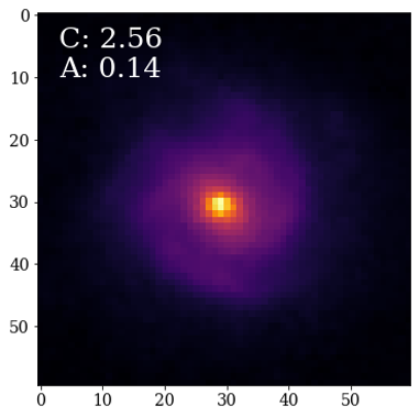
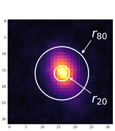
One of the most popular measurement's is the CAS system, which measures the concentration, asymmetry and smoothness of a galaxies light distribution.

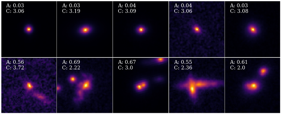
These parameters were found to correlate strongly with a galaxies past and ongoing formation modes and are hence useful as a robust classification system.

It has been shown that the concentration parameter correlates with the bulge-to-disk ratio (B/D) of a galaxy, while the asymmetry parameter is a good indicator of the merger history of the galaxy.

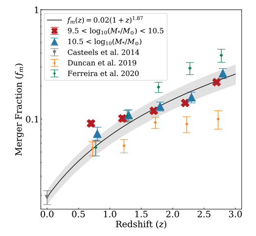
**Figure 2:** Merger fraction of galaxies in the CANDELS fields calculated using the asymmetry (A) parameter (Whitney et al. 2021).

**Figure 3:** Relationship between the concentration parameter (C) and the bulge to total light ratio (B/T) of a galaxy (Conselice 2003).

These parameters are simple in definition however, in practice require careful data cleaning and iterative processes. When we scale this up to future large-scale surveys such as Euclid and LSST, the amount of data that we are going to be collecting makes computing these parameters computationally expensive.

What we need to have in place is a more efficient and robust method for computing these parameters.

Solution? Machine learning! ML has already been successfully applied to other structural measurements such as the sersic profiles of galaxies (Tuccillo et al 2018).

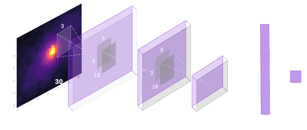
In this work we want to train Convolutional Neural networks to predict both the concentration and asymmetry of a galaxy from a single image.

The work presented in this poster is based on results from Tohill et al. 2021.

2. Concentration and Asymmetry

Concentration

The Concentration (C) parameter is simply a measure of how concentrated the light from the central region of a galaxy is compared to the outer parts. This can tell us if a galaxy has a disk structure, is more elliptical, or is an irregular type galaxy. In this way it correlates with the B/T light ratio of the galaxy.

It is calculated using the ratio of two radii that contain a predefined amount of light from the galaxy. For our measurements we use the ratio of the radii containing 80% and 20% of the total light.

Asymmetry

The Asymmetry (A) value is a measure of how asymmetric the galaxy light is, meaning galaxies that are undergoing a merging event with another galaxy will have high A values most of the time. The A value of a large sample of galaxies can then be used to estimate the merger fraction which is important in galaxy evolution models.

It is calculated by rotating the image 180° and subtracting it from the pre-rotated image. The residuals are then summed and divided by the original galaxy flux.

A = \frac{\sum|I - I_{180}|}{I} - A_\mathrm{bkg}\,

C = 5\log_{10} \left(\frac{r_{80}}{r_{20}} \right)

**Figure 4:** Graphical representation of how concentration is measured.

Data

We trained our networks using real data from the CANDELS fields (COSMOS, UDS, EGS, GOODS North and GOODS South) as imaged by the Hubble space telescope.

In total we had ~100,000 images 0.1 < z < 7. We use imaging from the H-band as it provides the most complete deep-coverage over all five CANDELS fields.

As this is a supervised task, we need labels for our data. We utilised an algorithm called Morfometryka to measure the C and A for all of the galaxies in our sample. An example of some of the galaxies in our sample are shown in the figure below. The concentration and asymmetry values are indicated in each stamp.

**Figure 5:** *Top row:* Images of the galaxies with high concentration values. These galaxies appear to be compact, spheroidal and have no close neighbours. *Bottom row:* Images of galaxies with high asymmetry values. Many of these galaxies appear to be undergoing mergers and have tidal effects present, although there are occasional cases of line-of-sight projection. The concentration (C) and asymmetry (A) are indicated above each galaxy stamp.

3. Machine Learning: Convolutional Neural Networks (CNNs)

The idea behind machine learning (ML) and artificial intelligence is the ability to teach a machine to ‘think’ like the human brain does. This is achieved by using a large amount of data to train the machine. This allows the machine to learn and improve without being explicitly programmed.

Within our work we utilise a type of deep learning network known as a Convolutional Neural Network (CNNs). These are networks that are best suited for image classification problems. CNNs are made up of convolutional layers which extract and learn features from images by applying multiple filter matrices to the image (see figure). These filters can extract features like shape, size, edges etc.

Machine learning has been used in many areas of astronomy ranging from galaxy classification (Dieleman et al. 2015; Cheng et al 2020) to merger detection (Ferreira et al. 2020).

**Figure 6:** Architecture of a convolutional neural network that takes a galaxy image as the input and outputs a single value corresponding to that galaxy. This is either the concentration or asymmetry value for our network.

ML has several advantages over previous computational methods including:

Much more efficient – our networks are ~10,000 times faster than the original algorithm.
Can improve over time with more data
Less susceptible to human bias (still have this bias with labelled data sometimes)
Requires fewer pre-processing steps as feature extraction and classification are preformed within the network.

4. Results

Trained networks

Our networks measurments correlate strongly with the conventionally measured values for both the concentration and asymmetry. The average difference between the conventionally measured values and our networks' predictions are lower than the typical error on each measurment.

To evaluate how well our networks are performing we compute the mean absolute error (MAE) and root mean squared error (RMSE) of the network's predictions. The RMSE metric also serves as our loss function. The MAE is simply a measure of the average magnitude of error between the network's prediction and the expected result. These are shown in the following equations, where n is the number of samples, y_i is the expected value and z_i is the network's prediction. The RMSE is similar to the MAE, but it is more sensitive to large errors and so can indicate if there are many outliers present.

\begin{equation} \mathrm{MAE} = \frac{1}{n} \sum_{i=1}^{n} |y_i - z_i|\,, \end{equation}

\begin{equation} \mathrm{RMSE} = \sqrt{\frac{1}{n} \sum_{i=1}^{n} {(y_i - z_i)}^2}\,. \end{equation}

**Figure 7:** Our final network’s predictions of concentration values for the test set versus those measured by Morfometryka. The MAE of the network was 0.15, with a RMSE of 0.21.

**Figure 8:** Our final network’s predictions of the asymmetries for the test set versus those measured by Morfometryka. The MAE of the network was 0.045, with a RMSE of 0.065.

From these results we can conclude that our networks can measure these parameters just as well as the direct measurements. Hence the values from the network can be utilised with a similar level of confidence as the original algorithm.

Impact of noise

Looking at the images of galaxies where there was a large difference between our networks and the Morfometryka-measured CAS values, we find that they are quite noisy, with signal to noise ratios (SNR) < 4.

**Figure 9:** Fractional residuals of the concentration network and the measured values from Morfometryka versus the SNR_p of each galaxy image. Black crosses represent the means in each bin with the darker shaded region representing ± 1 standard deviation.

**Figure 10:** Residuals of the asymmetry network and the measured values from Morfometryka versus the SNRp of each galaxy image. Black crosses represent the means in each bin with the darker shaded region representing ± 1 standard deviation.

Looking at the residuals as a function of SNR_p we can see that there is a trend where, at the low SNR_plevels our networks will on average slightly under-predict the values measured by the standard algorithms.

In order to determine if this low signal-to-noise trend is a bias in our networks or in the standard algorithm (as implemented in Morfometryka), we investigate how noise impacts these two approaches in an independent manner (see section 5).

5. Robustness and efficiency

Noise

To independently test the impact of noise on both our networks and the standard algorithm we preform a series of simulations.

We select a sub-sample of ~600 high SNR_p (SNR_p> 10) and simulate how these galaxies would appear at various SNR_plevels from 10 to 1. An example of one of these galaxies can be seen below.

**Figure 11:** An example of our simulated noisy galaxy images. The top-left panel shows the original image, while the remainder show the same galaxy at different simulated SNR_p.

We then remeasure both the C and A values of each galaxy at each SNR_plevel with both our networks and the standard algorithm and investigate how much these deviate from the 'true' values.

**Figure 12:** *Top:* Deviation in the asymmetry measurements from Morfometryka as the SNR_pdecreases. Black points indicate the mean residual at each bin, with error-bars showing ±1 standard deviation. *Bottom:* As the top panel, but for our trained network.

**Figure 13:** *Top:* Deviation in the concentration measurements from Morfometryka as the SNR_p decreases. Black points indicate the mean residual at each bin, with error-bars showing ±1 standard deviation. *Bottom:* As the top panel, but for our trained network.

Looking at the results for both concentration and asymmetry, it can be seen that at low SNR_plevels, both our networks and the standard algorithm have a bias where they will on average overestimate the values. This bias however, is much lower for our networks than the standard algorithm with the values recovered from our networks also being more accurate at the moderate to high SNR_plevels. Furthermore the scatter in the individual measurements are significantly lower for our networks as well.

These results suggest that our networks are using information in these moderate to low SNR_pimages that is not utilised by the Morfometryka algorithm. While there is scatter in the individual measurements, on average our network is able to accurately estimate both asymmetry and concentration, with little bias from the ‘true’ value, at a lower SNRp than the original algorithm.

This is useful for merger fraction estimates, especially at high redshift, as we can now include galaxy images down to a SNR_p as low as 3 while still retrieving unbiased measurements with our network.

This means that we are able to measure reliable CAS parameters for more galaxies using deep learning and then we can with a direct measurement.

Computational efficiency

Running both our trained networks and Morfometryka on a single computational core, for comparision, our networks are ~ 3,000 times faster. However, for a modern workstation, containing a single high-end consumer GPU (e.g. an NVIDIA GeForce GTX 1080 Ti) and 16 CPU cores, the results are even more striking. On such a system, our trained networks can analyse ∼ 10,000 galaxies in under 1.5 seconds, while it would take 2 hours to perform these measurements using the Morfometryka code.

The future of extragalactic astronomy consists of ‘Big Data’ surveys, which will image billions of galaxies. Current state of the art computational methods for analysing these surveys will become impractical due to the computational resources and time they need. While detailed analyses will be required for certain measurements, machine learning techniques can replace many current algorithms. CNN-based approaches are more efficient and, as we have shown for measuring CAS parameters, can be more accurate and reliable than traditional measurements. Measuring non-parametric morphologies in upcoming galaxy surveys, including those by the Euclid, Rubin, and Roman observatories, will greatly benefit from the methods presented in this work.